如何用 Python 追踪 NBA 球员的移动轨迹，pythonnba,未经许可，禁止转载！英文

文章由Byrx.net分享于2019-03-23 10:03:21评论（442）

如何用 Python 追踪 NBA 球员的移动轨迹，pythonnba,未经许可，禁止转载！英文

本文由编橙之家 - Sam Lin 翻译，黄利民校稿。未经许可，禁止转载！
英文出处：Savvas Tjortjoglou。欢迎加入翻译组。

在这篇文章中，我介绍了如何从 stats.nba.com 上现场实况运动动画中提取一些额外的信息。

In [1]:

Python

import requests
import pandas as pd
import numpy as np

%matplotlib inline
import matplotlib.pyplot as plt
import seaborn as sns

from IPython.display import IFrame

In [2]:

Python

sns.set_color_codes()
sns.set_style("white")

我们将会提取季后赛快船和火箭系列赛第 5 场比赛中一个回合的信息。在那个回合中，James Harden 突破到篮下，撕破快船的防守，然后传球给 Trevor Ariza，后者投入一个空位 3 分球。

我按照下面的方法嵌入运动动画。

In [3]:

Python

IFrame('http://stats.nba.com/movement/#!/?GameID=0041400235&amp;GameEventID=308',
              width=700, height=400)

Out[3]:

获取数据

通过下面的 URL，我们可以连接从 stats.nba.com API 得到的数据。在 URL 中有两个参数。eventid 是这个特定回合的 ID 号。gameid 是这场季后赛的 ID 号。

In [4]:

Python

url = "http://stats.nba.com/stats/locations_getmoments/?eventid=308&amp;gameid=0041400235"

下面将会使用 requests 来获取数据

In [5]:

Python

# Get the webpage
response = requests.get(url)
# Take a look at the keys from the dict
# representing the JSON data
response.json().keys()

Out[5]:

Python

dict_keys(['visitor', 'gamedate', 'moments', 'gameid', 'home'])

我们想要的数据可以在 home（主场球员的数据）、visitors（客场球员的数据）和 moments（包含上面用来绘制球员运动动画信息的数据）中找到。

In [6]:

Python

# A dict containing home players data
home = response.json()["home"]
# A dict containig visiting players data
visitor = response.json()["visitor"]
# A list containing each moment
moments = response.json()["moments"]

下面看一下字典 home 包含的信息。

In [7]:

Python

home

Out[7]:

Python

{'abbreviation': 'HOU',
 'name': 'Houston Rockets',
 'players': [{'firstname': 'Trevor',
   'jersey': '1',
   'lastname': 'Ariza',
   'playerid': 2772,
   'position': 'F'},
  {'firstname': 'Nick',
   'jersey': '3',
   'lastname': 'Johnson',
   'playerid': 203910,
   'position': 'G'},
  {'firstname': 'Josh',
   'jersey': '5',
   'lastname': 'Smith',
   'playerid': 2746,
   'position': 'F'},
  {'firstname': 'Terrence',
   'jersey': '6',
   'lastname': 'Jones',
   'playerid': 203093,
   'position': 'F'},
  {'firstname': 'Joey',
   'jersey': '8',
   'lastname': 'Dorsey',
   'playerid': 201595,
   'position': 'C-F'},
  {'firstname': 'Pablo',
   'jersey': '9',
   'lastname': 'Prigioni',
   'playerid': 203143,
   'position': 'G'},
  {'firstname': 'Dwight',
   'jersey': '12',
   'lastname': 'Howard',
   'playerid': 2730,
   'position': 'C'},
  {'firstname': 'James',
   'jersey': '13',
   'lastname': 'Harden',
   'playerid': 201935,
   'position': 'G'},
  {'firstname': 'Clint',
   'jersey': '15',
   'lastname': 'Capela',
   'playerid': 203991,
   'position': 'C'},
  {'firstname': 'Kostas',
   'jersey': '16',
   'lastname': 'Papanikolaou',
   'playerid': 203123,
   'position': 'F'},
  {'firstname': 'Jason',
   'jersey': '31',
   'lastname': 'Terry',
   'playerid': 1891,
   'position': 'G'},
  {'firstname': 'KJ',
   'jersey': '32',
   'lastname': 'McDaniels',
   'playerid': 203909,
   'position': 'G-F'},
  {'firstname': 'Corey',
   'jersey': '33',
   'lastname': 'Brewer',
   'playerid': 201147,
   'position': 'G-F'}],
 'teamid': 1610612745}

visitor 字典包含了同类信息，不过它是关于快船队的信息。

In [8]:

Python

visitor

Out[8]:

Python

{'abbreviation': 'LAC',
 'name': 'Los Angeles Clippers',
 'players': [{'firstname': 'Glen',
   'jersey': '0',
   'lastname': 'Davis',
   'playerid': 201175,
   'position': 'F-C'},
  {'firstname': 'Chris',
   'jersey': '3',
   'lastname': 'Paul',
   'playerid': 101108,
   'position': 'G'},
  {'firstname': 'JJ',
   'jersey': '4',
   'lastname': 'Redick',
   'playerid': 200755,
   'position': 'G'},
  {'firstname': 'DeAndre',
   'jersey': '6',
   'lastname': 'Jordan',
   'playerid': 201599,
   'position': 'C'},
  {'firstname': 'Spencer',
   'jersey': '10',
   'lastname': 'Hawes',
   'playerid': 201150,
   'position': 'F-C'},
  {'firstname': 'Jamal',
   'jersey': '11',
   'lastname': 'Crawford',
   'playerid': 2037,
   'position': 'G'},
  {'firstname': 'Ekpe',
   'jersey': '13',
   'lastname': 'Udoh',
   'playerid': 202327,
   'position': 'F'},
  {'firstname': 'Lester',
   'jersey': '14',
   'lastname': 'Hudson',
   'playerid': 201991,
   'position': 'G'},
  {'firstname': 'Hedo',
   'jersey': '15',
   'lastname': 'Turkoglu',
   'playerid': 2045,
   'position': 'F'},
  {'firstname': 'Matt',
   'jersey': '22',
   'lastname': 'Barnes',
   'playerid': 2440,
   'position': 'F'},
  {'firstname': 'Austin',
   'jersey': '25',
   'lastname': 'Rivers',
   'playerid': 203085,
   'position': 'G'},
  {'firstname': 'Dahntay',
   'jersey': '31',
   'lastname': 'Jones',
   'playerid': 2563,
   'position': 'G-F'},
  {'firstname': 'Blake',
   'jersey': '32',
   'lastname': 'Griffin',
   'playerid': 201933,
   'position': 'F'}],
 'teamid': 1610612746}

下面看看 moments 列表的内容。

In [9]:

Python

# Check the length
len(moments)

Out[9]:

Python

从长度可知上述的动画是由 700 个项/时刻组成。但是这些时刻包括了什么信息呢？让我们看下第一个时刻。

In [10]:

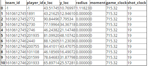
Python

moments[0]

Out[10]:

Python

[3,
 1431486313010,
 715.32,
 19.0,
 None,
 [[-1, -1, 43.51745, 10.76997, 1.11823],
  [1610612745, 1891, 43.21625, 12.9461, 0.0],
  [1610612745, 2772, 90.84496, 7.79534, 0.0],
  [1610612745, 2730, 77.19964, 34.36718, 0.0],
  [1610612745, 2746, 46.24382, 21.14748, 0.0],
  [1610612745, 201935, 81.0992, 48.10742, 0.0],
  [1610612746, 2440, 88.12605, 11.23036, 0.0],
  [1610612746, 200755, 84.41011, 43.47075, 0.0],
  [1610612746, 101108, 46.18569, 16.49072, 0.0],
  [1610612746, 201599, 78.64683, 31.87798, 0.0],
  [1610612746, 201933, 65.89714, 25.57281, 0.0]]]

首先，在 moments 里的时刻或者项是一个包含一堆信息的列表。下面我们一个一个地查看列表里的项。

moments[0] 的第一项是这个时刻发生的时期或者节（一场篮球比赛分为 4 节）
我不知道第二项代表什么。如果你知道的话请告诉我。
第三项是比赛用时钟剩下的时间。
第四项是投篮时限钟剩下的时间。
我不知道第五项代表什么。
第六项是由 11 个列表组成的列表，每个列表包含一个球员在球场中的坐标或者篮球的坐标。

1.这 11 个列表的第一个列表包含篮球的信息。

1.开始的两项代表 teamid 和 playerid 值，这两个值标识这个列表为篮球。
2.接下来的两项是 x 和 y 值，这两个值代表在球场上篮球的位置。
3.第五项代表篮球的半径。根据球的高度，这个值在动画的过程中始终是改变的。半径越大，球越高。所以如果一个球员投篮，球会变大，在投球弧线的顶点达到最大的尺寸，然后随着球下降，它的尺寸也变小。

2.列表第六项中，随后的 10 个列表代表球场上的 10 个球员。这些列表的信息与篮球的信息一样。

1.开始的两项是 teamid 和 playerid，这两个值标识这个列表为某个特定的球员。
2.接下来的两项代表球场上球员位置的 x 和 y 坐标值。
3.最后一项是球员的半径，该值无关紧要。

现在我们对 moments 数据的含义已有所了解，接下来将它放到 pandas DataFrame 中。

首先我们为 DataFrame 创建列标签。

In [11]:

Python

# Column labels
headers = ["team_id", "player_id", "x_loc", "y_loc", 
           "radius", "moment", "game_clock", "shot_clock"]

然后，我们单独创建一个列表，用于保存每个球员的 moments 数据。

In [12]:

Python

# Initialize our new list
player_moments = []

for moment in moments:
    # For each player/ball in the list found within each moment
    for player in moment[5]:
        # Add additional information to each player/ball
        # This info includes the index of each moment, the game clock
        # and shot clock values for each moment
        player.extend((moments.index(moment), moment[2], moment[3]))
        player_moments.append(player)

In [13]:

Python

# inspect our list
player_moments[0:11]

Out[13]:

Python

[[-1, -1, 43.51745, 10.76997, 1.11823, 0, 715.32, 19.0],
 [1610612745, 1891, 43.21625, 12.9461, 0.0, 0, 715.32, 19.0],
 [1610612745, 2772, 90.84496, 7.79534, 0.0, 0, 715.32, 19.0],
 [1610612745, 2730, 77.19964, 34.36718, 0.0, 0, 715.32, 19.0],
 [1610612745, 2746, 46.24382, 21.14748, 0.0, 0, 715.32, 19.0],
 [1610612745, 201935, 81.0992, 48.10742, 0.0, 0, 715.32, 19.0],
 [1610612746, 2440, 88.12605, 11.23036, 0.0, 0, 715.32, 19.0],
 [1610612746, 200755, 84.41011, 43.47075, 0.0, 0, 715.32, 19.0],
 [1610612746, 101108, 46.18569, 16.49072, 0.0, 0, 715.32, 19.0],
 [1610612746, 201599, 78.64683, 31.87798, 0.0, 0, 715.32, 19.0],
 [1610612746, 201933, 65.89714, 25.57281, 0.0, 0, 715.32, 19.0]]

将我们最新创建的 moments 列表传进 pd.DataFrame，和列标签一起创建 DataFrame。

In [14]:

Python

df = pd.DataFrame(player_moments, columns=headers)

In [15]:

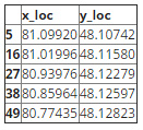
Python

df.head(11)

Out[15]:

我们还没完成。我们应该添加包含球员名字和球衣号码的列。首先将所有球员放到一个列表中。

In [16]:

Python

# creates the players list with the home players
players = home["players"]
# Then add on the visiting players
players.extend(visitor["players"])

使用 players 列表，我们可以创建一个字典，其中球员 ID 是字典的键，包含球员名字和球衣号码的列表作为字典的值。

In [17]:

Python

# initialize new dictionary
id_dict = {}

# Add the values we want
for player in players:
    id_dict[player['playerid']] = [player["firstname"]+" "+player["lastname"],
                                   player["jersey"]]

In [18]:

Python

id_dict

Out[18]:

Python

{1891: ['Jason Terry', '31'],
 2037: ['Jamal Crawford', '11'],
 2045: ['Hedo Turkoglu', '15'],
 2440: ['Matt Barnes', '22'],
 2563: ['Dahntay Jones', '31'],
 2730: ['Dwight Howard', '12'],
 2746: ['Josh Smith', '5'],
 2772: ['Trevor Ariza', '1'],
 101108: ['Chris Paul', '3'],
 200755: ['JJ Redick', '4'],
 201147: ['Corey Brewer', '33'],
 201150: ['Spencer Hawes', '10'],
 201175: ['Glen Davis', '0'],
 201595: ['Joey Dorsey', '8'],
 201599: ['DeAndre Jordan', '6'],
 201933: ['Blake Griffin', '32'],
 201935: ['James Harden', '13'],
 201991: ['Lester Hudson', '14'],
 202327: ['Ekpe Udoh', '13'],
 203085: ['Austin Rivers', '25'],
 203093: ['Terrence Jones', '6'],
 203123: ['Kostas Papanikolaou', '16'],
 203143: ['Pablo Prigioni', '9'],
 203909: ['KJ McDaniels', '32'],
 203910: ['Nick Johnson', '3'],
 203991: ['Clint Capela', '15']}

更新 id_dict 来包括球的 id。

In [19]:

Python

id_dict.update({-1: ['ball', np.nan]})

然后，在 player_id 列上使用 map 方法来创建一个 player_name 列和 player_jersey 列。我们将使用 lambda 创建一个匿名函数，该函数根据传进函数的 player_id 值返回正确的 player_name 和 player_jersey。

换句话说，下面代码做的事情是在 player_id 列中迭代球员的 ID，然后将每个球员 ID 传进匿名函数。这个函数会返回与球员 ID 相关联的球员名和球衣号码，并且将那些值添加到 DataFrame。

In [20]:

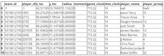
Python

df["player_name"] = df.player_id.map(lambda x: id_dict[x][0])
df["player_jersey"] = df.player_id.map(lambda x: id_dict[x][1])

In [21]:

Python

df.head(11)

Out[21]:

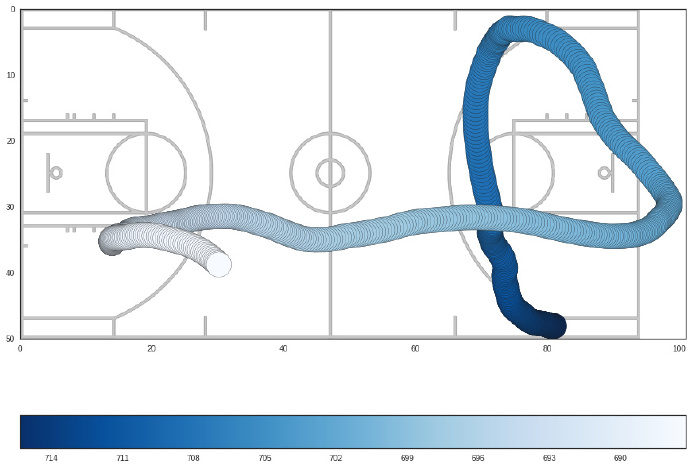
绘制移动轨迹

下面我们通过动画绘制 James Harden 的移动轨迹。我们可以使用从 stas.nba.com 得到的动画上画好的球场来绘制球场。你可以在这里找到 SVG 图片。我将它转换成一个 PNG 文件，这样可以更容易地使用 matplotlib 来绘制。也要注意 x 或者 y 轴上的每 1 个单位表示篮球场上的 1 英尺。

In [22]:

Python

# get Harden's movements
harden = df[df.player_name=="James Harden"]
# read in the court png file
court = plt.imread("fullcourt.png")

In [23]:

Python

plt.figure(figsize=(15, 11.5))

# Plot the movemnts as scatter plot
# using a colormap to show change in game clock
plt.scatter(harden.x_loc, harden.y_loc, c=harden.game_clock,
            cmap=plt.cm.Blues, s=1000, zorder=1)
# Darker colors represent moments earlier on in the game
cbar = plt.colorbar(orientation="horizontal")
cbar.ax.invert_xaxis()

# This plots the court
# zorder=0 sets the court lines underneath Harden's movements
# extent sets the x and y axis values to plot the image within.
# The original animation plots in the SVG coordinate space
# which has x=0, and y=0 at the top left.
# So, we set the axis values the same way in this plot.
# In the list we pass to extent 0,94 representing the x-axis 
# values and 50,0 representing the y-axis values
plt.imshow(court, zorder=0, extent=[0,94,50,0])

# extend the x-values beyond the court b/c Harden
# goes out of bounds
plt.xlim(0,101)

plt.show()

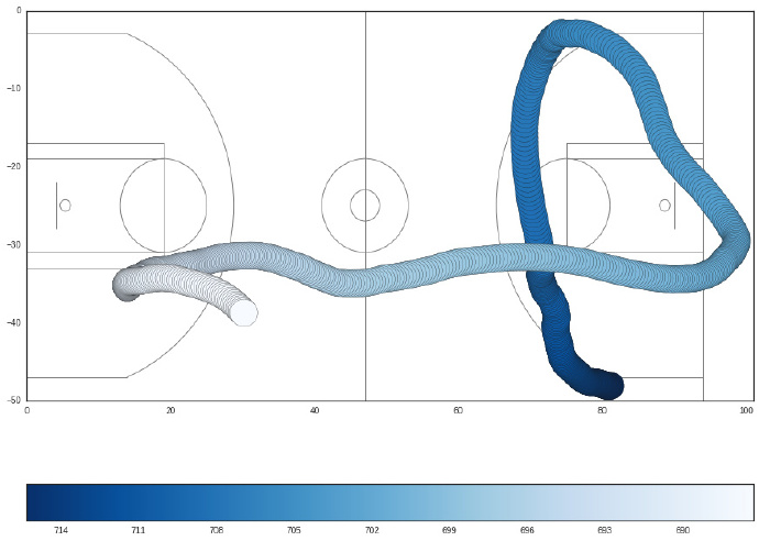
我们也可以仅使用 matplotlib Patches 来重新创建球场的大部分。我们使用传统的笛卡尔坐标系，而不使用 SVG 坐标系，所以 y 值将会是负数，而不是正数。

In [24]:

Python

from matplotlib.patches import Circle, Rectangle, Arc

# Function to draw the basketball court lines
def draw_court(ax=None, color="gray", lw=1, zorder=0):

    if ax is None:
        ax = plt.gca()

    # Creates the out of bounds lines around the court
    outer = Rectangle((0,-50), width=94, height=50, color=color,
                      zorder=zorder, fill=False, lw=lw)

    # The left and right basketball hoops
    l_hoop = Circle((5.35,-25), radius=.75, lw=lw, fill=False, 
                    color=color, zorder=zorder)
    r_hoop = Circle((88.65,-25), radius=.75, lw=lw, fill=False,
                    color=color, zorder=zorder)

    # Left and right backboards
    l_backboard = Rectangle((4,-28), 0, 6, lw=lw, color=color,
                            zorder=zorder)
    r_backboard = Rectangle((90, -28), 0, 6, lw=lw,color=color,
                            zorder=zorder)

    # Left and right paint areas
    l_outer_box = Rectangle((0, -33), 19, 16, lw=lw, fill=False,
                            color=color, zorder=zorder)    
    l_inner_box = Rectangle((0, -31), 19, 12, lw=lw, fill=False,
                            color=color, zorder=zorder)
    r_outer_box = Rectangle((75, -33), 19, 16, lw=lw, fill=False,
                            color=color, zorder=zorder)

    r_inner_box = Rectangle((75, -31), 19, 12, lw=lw, fill=False,
                            color=color, zorder=zorder)

    # Left and right free throw circles
    l_free_throw = Circle((19,-25), radius=6, lw=lw, fill=False,
                          color=color, zorder=zorder)
    r_free_throw = Circle((75, -25), radius=6, lw=lw, fill=False,
                          color=color, zorder=zorder)

    # Left and right corner 3-PT lines
    # a represents the top lines
    # b represents the bottom lines
    l_corner_a = Rectangle((0,-3), 14, 0, lw=lw, color=color,
                           zorder=zorder)
    l_corner_b = Rectangle((0,-47), 14, 0, lw=lw, color=color,
                           zorder=zorder)
    r_corner_a = Rectangle((80, -3), 14, 0, lw=lw, color=color,
                           zorder=zorder)
    r_corner_b = Rectangle((80, -47), 14, 0, lw=lw, color=color,
                           zorder=zorder)

    # Left and right 3-PT line arcs
    l_arc = Arc((5,-25), 47.5, 47.5, theta1=292, theta2=68, lw=lw,
                color=color, zorder=zorder)
    r_arc = Arc((89, -25), 47.5, 47.5, theta1=112, theta2=248, lw=lw,
                color=color, zorder=zorder)

    # half_court
    # ax.axvline(470)
    half_court = Rectangle((47,-50), 0, 50, lw=lw, color=color,
                           zorder=zorder)

    hc_big_circle = Circle((47, -25), radius=6, lw=lw, fill=False,
                           color=color, zorder=zorder)
    hc_sm_circle = Circle((47, -25), radius=2, lw=lw, fill=False,
                          color=color, zorder=zorder)

    court_elements = [l_hoop, l_backboard, l_outer_box, outer,
                      l_inner_box, l_free_throw, l_corner_a,
                      l_corner_b, l_arc, r_hoop, r_backboard, 
                      r_outer_box, r_inner_box, r_free_throw,
                      r_corner_a, r_corner_b, r_arc, half_court,
                      hc_big_circle, hc_sm_circle]

    # Add the court elements onto the axes
    for element in court_elements:
        ax.add_patch(element)

    return ax

In [25]:

Python

plt.figure(figsize=(15, 11.5))

# Plot the movemnts as scatter plot
# using a colormap to show change in game clock
plt.scatter(harden.x_loc, -harden.y_loc, c=harden.game_clock,
            cmap=plt.cm.Blues, s=1000, zorder=1)
# Darker colors represent moments earlier on in the game
cbar = plt.colorbar(orientation="horizontal")
# invert the colorbar to have higher numbers on the left
cbar.ax.invert_xaxis()

draw_court()

plt.xlim(0, 101)
plt.ylim(-50, 0)
plt.show()

计算移动距离

我们可以通过获取相邻点的欧氏距离计算出一个球员的移动距离，然后添加那些距离。

关于获取相邻点欧氏距离的链接。

In [26]:

Python

def travel_dist(player_locations):
    # get the differences for each column
    diff = np.diff(player_locations, axis=0)
    # square the differences and add them,
    # then get the square root of that sum
    dist = np.sqrt((diff ** 2).sum(axis=1))
    # Then return the sum of all the distances
    return dist.sum()

In [27]:

Python

# Harden's travel distance
dist = travel_dist(harden[["x_loc", "y_loc"]])
dist

Out[27]:

Python

197.44816608512659

我们可以使用 groupby 和 apply 得到每个球员总的移动距离。以球员分组，获取他们每个人的坐标位置，然后 apply 上面的 distance 函数。

In [28]:

Python

player_travel_dist = df.groupby('player_name')[['x_loc', 'y_loc']].apply(travel_dist)
player_travel_dist

Out[28]:

Python

player_name
Blake Griffin     153.076637
Chris Paul        176.198330
DeAndre Jordan    119.919877
Dwight Howard     123.439590
JJ Redick         184.504145
James Harden      197.448166
Jason Terry       173.308880
Josh Smith        162.226100
Matt Barnes       161.976406
Trevor Ariza      153.389365
ball              328.317612
dtype: float64

计算平均速度

计算一个球员的平均速度非常简单。我们只需以时间来划分距离。

In [29]:

Python

# get the number of seconds for the play
seconds = df.game_clock.max() - df.game_clock.min()
# feet per second
harden_fps = dist / seconds
# convert to miles per hour
harden_mph = 0.681818 * harden_fps
harden_mph

Out[29]:

Python

4.7977089702005902

我们可以使用之前创建的 player_travel_dist Series 来获取每个球员的平均速度。

In [30]:

Python

player_speeds = (player_travel_dist/seconds) * 0.681818
player_speeds

Out[30]:

Python

player_name
Blake Griffin     3.719544
Chris Paul        4.281368
DeAndre Jordan    2.913882
Dwight Howard     2.999406
JJ Redick         4.483188
James Harden      4.797709
Jason Terry       4.211159
Josh Smith        3.941863
Matt Barnes       3.935796
Trevor Ariza      3.727143
ball              7.977650
dtype: float64

计算球员之间的距离

下面将看下在比赛中，Harden 与其他每个球员之间的距离。

首先获取 Harden 的位置。

In [31]:

Python

harden_loc = df[df.player_name=="James Harden"][["x_loc", "y_loc"]]

In [32]:

Python

harden_loc.head()

Out[32]:

现在让我们以 player_name 进行分组，并且获取每个球员和篮球的位置。

In [33]:

Python

group = df[df.player_name!="James Harden"].groupby("player_name")[["x_loc", "y_loc"]]

我们可以利用 group 中 scipy 库的 euclidean 函数来 apply 一个函数。然后为每个球员返回一个列表，该列表包含比赛中 James Harden 与该球员之间的距离。

In [34]:

Python

from scipy.spatial.distance import euclidean

In [35]:

Python

# Function to find the distance between players
# at each moment
def player_dist(player_a, player_b):
    return [euclidean(player_a.iloc[i], player_b.iloc[i])
            for i in range(len(player_a))]

每个球员的位置以 player_a 传进 player_dist 函数中，而 Harden 的位置则以 player_b 传进该函数。

In [36]:

Python

harden_dist = group.apply(player_dist, player_b=(harden_loc))

In [37]:

Python

harden_dist

Out[37]:

Python

player_name
Blake Griffin     [27.182922508363593, 27.055820685362697, 26.94...
Chris Paul        [47.10168680005101, 46.861684798626264, 46.618...
DeAndre Jordan    [16.413678482610162, 16.48314022711995, 16.556...
Dwight Howard     [14.282883583198455, 14.35720390798292, 14.433...
JJ Redick         [5.697440979685529, 5.683098128626677, 5.67370...
Jason Terry       [51.685939334067434, 51.40228120171322, 51.096...
Josh Smith        [44.06513224475787, 43.81023267813696, 43.5637...
Matt Barnes       [37.5405670597302, 37.59395273374297, 37.68516...
Trevor Ariza      [41.47340873263252, 41.414794206955804, 41.348...
ball              [52.976156009708745, 52.70430545836839, 52.435...
dtype: object

注意到篮球的列表中只有 690 项，而球员的则有 700 项。

In [38]:

Python

len(harden_dist["ball"])

Out[38]:

Python

In [39]:

Python

len(harden_dist["Blake Griffin"])

Out[39]:

Python

现在我们知道如何得到球员之间的距离，接下来让我们试着看下 James Harden 突破到篮底是如何影响地板上的一些间距。

让我们再看看 moments 动画。然后仔细查看在 Harden 突破期间会出现什么。

In [40]:

Python

IFrame('http://stats.nba.com/movement/#!/?GameID=0041400235&amp;GameEventID=308',
              width=700, height=400)

Out[40]:

当 Harden 突破到篮框时，DeAndre Jordan 从 Dwight Howards 旁离开去防守篮框，而 Matt Barnes 轮换来挡住 Howards（但是摔倒了），留给 Ariza 空位。Harden 看到 Ariza，传球给他，在 Chris Paul 尝试冲过来防守的同时，Ariza 投篮了。所有的这些发生在从距离第三节结束还有 11:46 到 11:42 分钟期间，而投篮时限钟从 Harden 开始突破的 10.1 秒跑到 Ariza 投出篮球的 6.2 秒。实际上我们可以在 Ariza 的投篮日志页面中找到更多关于 Ariza 投篮尝试的信息。

In [41]:

Python

# Boolean mask used to grab the data within the proper time period
time_mask = (df.game_clock &lt;= 706) &amp; (df.game_clock &gt;= 702) &amp; 
            (df.shot_clock &lt;= 10.1) &amp; (df.shot_clock &gt;= 6.2)
time_df = df[time_mask]

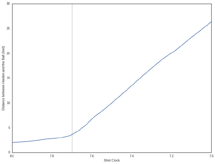
从动画中，看上去 Harden 在进攻时间剩下大约 7.7 到 7.8 秒的时候传球的。我们可以仔细查看他和球之间的距离来确定。

In [42]:

Python

ball = time_df[time_df.player_name=="ball"]
harden2 = time_df[time_df.player_name=="James Harden"]
harden_ball_dist = player_dist(ball[["x_loc", "y_loc"]],
                               harden2[["x_loc", "y_loc"]])

In [43]:

Python

plt.figure(figsize=(12,9))

x = time_df.shot_clock.unique()
y =  harden_ball_dist
plt.plot(x, y)
plt.xlim(8, 7)

plt.xlabel("Shot Clock")
plt.ylabel("Distance between Harden and the Ball (feet)")
plt.vlines(7.7, 0, 30, color='gray', lw=0.7)

plt.show()

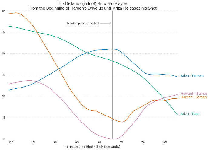
下面将绘制在这期间，一些球员之间距离的变化。我们将会绘制 Harden 和 Jordan、Howard 和 Barnes、Ariza 和 Barnes 以及 Ariza 和 Paul 之间距离的变化。

In [44]:

Python

# Boolean mask to get the players we want
player_mask = (time_df.player_name=="Trevor Ariza") | 
              (time_df.player_name=="DeAndre Jordan") | 
              (time_df.player_name=="Dwight Howard") | 
              (time_df.player_name=="Matt Barnes") | 
              (time_df.player_name=="Chris Paul") | 
              (time_df.player_name=="James Harden")

In [45]:

Python

# Group by players and get their locations
group2 = time_df[player_mask].groupby('player_name')[["x_loc", "y_loc"]]

In [46]:

Python

# Get the differences in distances that we want
harden_jordan = player_dist(group2.get_group("James Harden"),
                            group2.get_group("DeAndre Jordan"))
howard_barnes = player_dist(group2.get_group("Dwight Howard"),
                            group2.get_group("Matt Barnes"))
ariza_barnes = player_dist(group2.get_group("Trevor Ariza"),
                            group2.get_group("Matt Barnes"))
ariza_paul = player_dist(group2.get_group("Trevor Ariza"),
                            group2.get_group("Chris Paul"))

In [47]:

Python

# Create some lists that will help create our plot
# Distance data
distances = [ariza_barnes, ariza_paul, harden_jordan, howard_barnes]
# Labels for each line that we will plopt
labels = ["Ariza - Barnes", "Ariza - Paul", "Harden - Jordan", "Howard - Barnes"]
# Colors for each line
colors = sns.color_palette('colorblind', 4)

plt.figure(figsize=(12,9))

# Use enumerate to index the labels and colors and match
# them with the proper distance data
for i, dist in enumerate(distances):
    plt.plot(time_df.shot_clock.unique(), dist, color=colors[i])

    y_pos = dist[-1]

    plt.text(6.15, y_pos, labels[i], fontsize=14, color=colors[i])

# Plot a line to indicate when Harden passes the ball
plt.vlines(7.7, 0, 30, color='gray', lw=0.7)
plt.annotate("Harden passes the ball", (7.7, 27), 
             xytext=(8.725, 26.8), fontsize=12, 
             arrowprops=dict(facecolor='lightgray', shrink=0.10))

# Create horizontal grid lines
plt.grid(axis='y',color='gray', linestyle='--', lw=0.5, alpha=0.5)

plt.xlim(10.1, 6.2)

plt.title("The Distance (in feet) Between Players nFrom the Beginning"
          " of Harden's Drive up until Ariza Releases his Shot", size=16)
plt.xlabel("Time Left on Shot Clock (seconds)", size=14)

# Get rid of unneeded chart lines
sns.despine(left=True, bottom=True) 

plt.show()

我创建了一个小的 Python 模块，你可以在这里找到，里面包含了本文用过的一些函数。

打赏支持我翻译更多好文章，谢谢！
打赏译者

打赏支持我翻译更多好文章，谢谢！

热门文章：

如何用 Python 追踪 NBA 球员的移动轨迹，pythonnba,未经许可，禁止转载！英文