局部加权之逻辑回归(1) - Python实现，,算法特征:利用sig

局部加权之逻辑回归(1) - Python实现，,算法特征:利用sig

算法特征:
利用sigmoid函数的概率含义, 借助回归之手段达到分类之目的.算法推导:
Part Ⅰ
sigmoid函数之定义:
\begin{equation}\label{eq_1}
sig(x) = \frac{1}{1 + e^{-x}}
\end{equation}
相关函数图像:
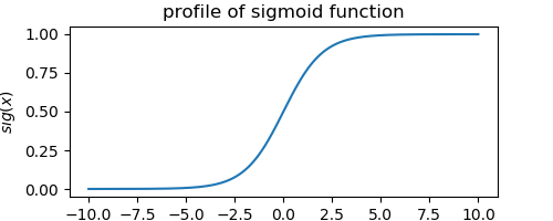由此可见, sigmoid函数将整个实数域$(-\infty, +\infty)$映射至$(0, 1)$区间内, 反映了一种良好概率意义下的映射关系. 对该函数进行如下扩展:
\begin{equation}\label{eq_2}
sig(\theta(x)) = \frac{1}{1 + e^{-\theta(x)}}
\end{equation}
其中, $x$为输入参数, $\theta(x)$为sigmoid函数之相位. 展开该相位, 可获取sigmoid函数之特征线$\theta(x) = c$, 特征线$\theta(x) = 0$也就是我们最常见的分界线.很显然, 相位$\theta(x)$之具体形式将影响分界线最终的表达能力, 即分界线形状的复杂程度.
为避免混淆, 现将相位$\theta(x)$拆开:①. $x$ ~ 输入参数;②. $\theta$ ~ 相位参数.在具有严格数理要求的情形下, 相位参数按实际要求选取; 否则, 经过训练集上的交叉验证选择合适的形式即可.

Part Ⅱ
现建立如下假设模型:
\begin{equation}\label{eq_4}
h_{\theta}(x) = sig(\theta(x))
\end{equation}
以$y = 1$表示正例, $y = 0$表示负例. 令$h_{\theta}(x)$表示输入参数$x$取正例之概率, $1 - h_{\theta}(x)$表示输入参数$x$取负例之概率, 则假设模型对输入参数$x$预测正确之概率(正例情况下预测正例之概率、负例情况下预测负例之概率)为:
\begin{equation}\label{eq_5}
P(right \mid x, \theta) = h_{\theta}(x)^y(1 - h_{\theta}(x))^{(1 - y)}
\end{equation}
考虑训练集中存在$n$个样本, 假设相位参数$\theta$已知, 则此n个样本同时预测正确之概率为:
\begin{equation}\label{eq_6}
L(\theta) =\prod_{i = 1}^{n}P(right \mid x^{(i)}, \theta)
\end{equation}
对该似然函数取对数似然:
\begin{equation}\label{eq_7}
lnL(\theta) = \sum_{i = 1}^{n}lnP(right \mid x^{(i)}, \theta)
\end{equation}
定义损失函数:
\begin{equation}\label{eq_8}
J(\theta) = -\frac{1}{n}lnL(\theta)
\end{equation}
根据最大似然估计, 有如下无约束最优化问题:
\begin{equation}\label{eq_9}
min\ J(\theta)
\end{equation}
其中, 相位参数$\theta$为优化变量. 对该优化问题进行求解, 即可获取相位参数$\theta$之最优解, 也即当前训练集下的最优分类模型.

Part Ⅲ
为方便优化, 给出如下协助信息:
\begin{equation}\label{eq_10}
\left\{\begin{matrix}
\nabla h_{\theta} = h_{\theta}(1 - h_{\theta})\nabla \theta \\
\nabla lnh_{\theta} = (1 - h_{\theta})\nabla \theta \\
\nabla ln(1 - h_{\theta}) = -h_{\theta}\nabla \theta
\end{matrix}\right.
\end{equation}
目标函数$J(\theta)$之gradient:
\begin{equation}\label{eq_11}
\nabla J = -\frac{1}{n} \sum_{i = 1}^{n} (y^{(i)} - h_{\theta}(x^{(i)}))\nabla \theta \\
\end{equation}
目标函数$J(\theta)$之Hessian矩阵:
\begin{equation}\label{eq_12}
H = \nabla^2 J = -\frac{1}{n} \sum_{i = 1}^{n}[(y^{(i)} - h_{\theta}(x^{(i)}))\nabla^2 \theta - h_{\theta}(x^{(i)})(1 - h_{\theta}(x^{(i)}))\nabla \theta (\nabla \theta)^T]
\end{equation}

Part Ⅳ
引入局部加权项$exp(-\left \| x_i - x\right \|_2^2 / (2\tau^2))$, 引入原则:
①. 不改变损失函数$J(\theta)$中各样本的损失贡献计算方式;
②. 对样本的损失贡献独立进行加权.
③. 泛化误差之计算仅依赖于样本的损失贡献.

Part Ⅴ
现以一个二分类为例进行算法实施.
以常见的$\theta(x) = 0$作为分界线, 并令:
\begin{equation}
\left\{\begin{matrix}
h_{\theta}(x) \geq 0.5 & y = 1 & 正例 \\
h_{\theta}(x) < 0.5 & y = 0 & 负例
\end{matrix}\right.
\end{equation}代码实现:

  1 # 局部加权之逻辑回归  2   3 import numpy  4 from matplotlib import pyplot as plt  5   6   7 def spiral_point(val, center=(0.5, 0.5)):  8     rn = 0.4 * (105 - val) / 104  9     an = numpy.pi * (val - 1) / 25 10      11     x0 = center[0] + rn * numpy.sin(an) 12     y0 = center[1] + rn * numpy.cos(an) 13     z0 = 0 14     x1 = center[0] - rn * numpy.sin(an) 15     y1 = center[1] - rn * numpy.cos(an) 16     z1 = 1 17      18     return (x0, y0, z0), (x1, y1, z1) 19  20  21 def spiral_data(valList): 22     dataList = list(spiral_point(val) for val in valList) 23     data0 = numpy.array(list(item[0] for item in dataList)) 24     data1 = numpy.array(list(item[1] for item in dataList)) 25     return data0, data1 26  27  28 # 生成训练数据集 29 trainingValList = numpy.arange(1, 101, 1) 30 trainingData0, trainingData1 = spiral_data(trainingValList) 31 trainingSet = numpy.vstack((trainingData0, trainingData1)) 32  33 # 生成测试数据集 34 testValList = numpy.arange(1.5, 101.5, 1) 35 testData0, testData1 = spiral_data(testValList) 36 testSet = numpy.vstack((testData0, testData1)) 37  38  39 # 假设模型 40 def h_theta(x, theta): 41     val = 1. / (1. + numpy.exp(-numpy.sum(x * theta))) 42     return val 43  44  45 # 假设模型预测正确之概率 46 def p_right(x, y_, theta): 47     val = h_theta(x, theta) ** y_ * (1. - h_theta(x, theta)) ** (1 - y_) 48     return val 49  50      51 # 加权损失函数 52 def JW(X, Y_, W, theta): 53     JVal = 0 54     for colIdx in range(X.shape[1]): 55         x = X[:, colIdx:colIdx+1] 56         y_ = Y_[colIdx, 0] 57         w = W[colIdx, 0] 58         pVal = p_right(x, y_, theta) if p_right(x, y_, theta) >= 1.e-100 else 1.e-100 59         JVal += w * numpy.log(pVal) 60     JVal = -JVal / X.shape[1] 61     return JVal 62      63  64 # 加权损失函数之梯度 65 def JW_grad(X, Y_, W, theta): 66     grad = numpy.zeros(shape=theta.shape) 67     for colIdx in range(X.shape[1]): 68         x = X[:, colIdx:colIdx+1] 69         y_ = Y_[colIdx, 0] 70         w = W[colIdx, 0] 71         grad += w * (y_ - h_theta(x, theta)) * x 72     grad = -grad / X.shape[1] 73     return grad 74  75      76 # 加权损失函数之Hessian 77 def JW_Hess(X, Y_, W, theta): 78     Hess = numpy.zeros(shape=(theta.shape[0], theta.shape[0])) 79     for colIdx in range(X.shape[1]): 80         x = X[:, colIdx:colIdx+1] 81         y_ = Y_[colIdx, 0] 82         w = W[colIdx, 0] 83         Hess += w * h_theta(x, theta) * (1 - h_theta(x, theta)) * numpy.matmul(x, x.T) 84     Hess = Hess / X.shape[1] 85     return Hess 86  87      88 class LWLR(object): 89      90     def __init__(self, trainingSet, tauBound=(0.001, 0.1), epsilon=1.e-3): 91         self.__trainingSet = trainingSet                             # 训练集 92         self.__tauBound = tauBound                                   # tau之搜索边界 93         self.__epsilon = epsilon                                     # tau之搜索精度 94          95      96     def search_tau(self): 97         ‘‘‘ 98         交叉验证返回最优tau 99         采用黄金分割法计算最优tau100         ‘‘‘101         X, Y_ = self.__get_XY_(self.__trainingSet)102         lowerBound, upperBound = self.__tauBound103         lowerTau = self.__calc_lowerTau(lowerBound, upperBound)104         upperTau = self.__calc_upperTau(lowerBound, upperBound)105         lowerErr = self.__calc_generalErr(X, Y_, lowerTau)106         upperErr = self.__calc_generalErr(X, Y_, upperTau)107         108         while (upperTau - lowerTau) > self.__epsilon:109             if lowerErr > upperErr:110                 lowerBound = lowerTau111                 lowerTau = upperTau112                 lowerErr = upperErr113                 upperTau = self.__calc_upperTau(lowerBound, upperBound)114                 upperErr = self.__calc_generalErr(X, Y_, upperTau)115             else:116                 upperBound = upperTau117                 upperTau = lowerTau118                 upperErr = lowerErr119                 lowerTau = self.__calc_lowerTau(lowerBound, upperBound)120                 lowerErr = self.__calc_generalErr(X, Y_, lowerTau)121             # print("{}, {}~{}, {}~{}, {}".format(lowerBound, lowerTau, lowerErr, upperTau, upperErr, upperBound))122         self.bestTau = (upperTau + lowerTau) / 2123         # print(self.bestTau)124         return self.bestTau125         126     127     def __calc_generalErr(self, X, Y_, tau):128         cnt = 0129         generalErr = 0130         131         for idx in range(X.shape[1]):132             tmpx = X[:, idx:idx+1]133             tmpy_ = Y_[idx, 0]134             tmpX = numpy.hstack((X[:, 0:idx], X[:, idx+1:]))135             tmpY_ = numpy.vstack((Y_[0:idx, :], Y_[idx+1:, :]))136             tmpW = self.__get_W(tmpx, tmpX, tau)137             theta, tab = self.__optimize_theta(tmpX, tmpY_, tmpW)138             # print(idx, tab, tmpx.reshape(-1), tmpy_, h_theta(tmpx, theta), theta.reshape(-1))139             if not tab:140                 continue141             cnt += 1142             generalErr -= numpy.log(p_right(tmpx, tmpy_, theta))143         generalErr /= cnt144         # print(tau, generalErr)145         return generalErr146         147         148     def __calc_lowerTau(self, lowerBound, upperBound):149         delta = upperBound - lowerBound150         lowerTau = upperBound - delta * 0.618151         return lowerTau152         153         154     def __calc_upperTau(self, lowerBound, upperBound):155         delta = upperBound - lowerBound156         upperTau = lowerBound + delta * 0.618157         return upperTau158         159         160     def __optimize_theta(self, X, Y_, W, maxIter=1000, epsilon=1.e-9):161         ‘‘‘162         maxIter: 最大迭代次数163         epsilon: 收敛判据 ~ 梯度趋于0则收敛164         ‘‘‘165         theta = self.__init_theta((X.shape[0], 1))166         JVal = JW(X, Y_, W, theta)167         grad = JW_grad(X, Y_, W, theta)168         Hess = JW_Hess(X, Y_, W, theta)169         for i in range(maxIter):170             if self.__is_converged1(grad, epsilon):171                 return theta, True172             173             dCurr = -numpy.matmul(numpy.linalg.inv(Hess + 1.e-9 * numpy.identity(Hess.shape[0])), grad)174             alpha = self.__calc_alpha_by_ArmijoRule(theta, JVal, grad, dCurr, X, Y_, W)175             176             thetaNew = theta + alpha * dCurr177             JValNew = JW(X, Y_, W, thetaNew)178             if self.__is_converged2(thetaNew - theta, JValNew - JVal, epsilon):179                 return thetaNew, True180             181             theta = thetaNew182             JVal = JValNew183             grad = JW_grad(X, Y_, W, theta)184             Hess = JW_Hess(X, Y_, W, theta)185             # print(i, JVal, grad.reshape(-1))186         else:187             if self.__is_converged(grad, epsilon):188                 return theta, True189         190         return theta, False191         192     193     def __calc_alpha_by_ArmijoRule(self, thetaCurr, JCurr, gCurr, dCurr, X, Y_, W, c=1.e-4, v=0.5):194         i = 0195         alpha = v ** i196         thetaNext = thetaCurr + alpha * dCurr197         JNext = JW(X, Y_, W, thetaNext)198         while True:199             if JNext <= JCurr + c * alpha * numpy.matmul(dCurr.T, gCurr)[0, 0]: break200             i += 1201             alpha = v ** i202             thetaNext = thetaCurr + alpha * dCurr203             JNext = JW(X, Y_, W, thetaNext)204         205         return alpha206     207     208     def __is_converged1(self, grad, epsilon):209         if numpy.linalg.norm(grad) <= epsilon:210             return True211         return False212         213         214     def __is_converged2(self, thetaDelta, JValDelta, epsilon):215         if numpy.linalg.norm(thetaDelta) <= epsilon or numpy.linalg.norm(JValDelta) <= epsilon:216             return True217         return False218     219     220     def __init_theta(self, shape):221         ‘‘‘222         theta之初始化223         ‘‘‘224         thetaInit = numpy.zeros(shape=shape)225         return thetaInit226         227         228     def __get_XY_(self, dataSet):229         self.X = dataSet[:, 0:2].T                                                 # 注意数值溢出230         self.X = numpy.vstack((self.X, numpy.ones(shape=(1, self.X.shape[1]))))231         self.Y_ = dataSet[:, 2:3]232         return self.X, self.Y_233         234         235     def __get_W(self, x, X, tau):236         term1 = numpy.sum((X - x) ** 2, axis=0)237         term2 = -term1 / (2 * tau ** 2)238         term3 = numpy.exp(term2)239         W = term3.reshape(-1, 1)240         return W241         242         243     def get_cls(self, x, tau=None, midVal=0.5):244         if tau is None:245             if not hasattr(self, "bestTau"):246                 self.search_tau()247             tau = self.bestTau248         if not hasattr(self, "X"):249             self.__get_XY_(self.__trainingSet)250             251         tmpx = numpy.vstack((numpy.array(x).reshape(-1, 1), numpy.ones(shape=(1, 1))))   # 注意数值溢出252         tmpW = self.__get_W(tmpx, self.X, tau)253         theta, tab = self.__optimize_theta(self.X, self.Y_, tmpW)254         255         realVal = h_theta(tmpx, theta)256         if realVal > midVal:                   # 正例257             return 1258         elif realVal == midVal:                # 中间259             return 0.5260         else:                                  # 负例261             return 0262         263         264     def get_accuracy(self, testSet, tau=None, midVal=0.5):265         ‘‘‘266         正确率计算267         ‘‘‘268         if tau is None:269             if not hasattr(self, "bestTau"):270                 self.search_tau()271             tau = self.bestTau272         273         rightCnt = 0274         for row in testSet:275             cls = self.get_cls(row[:2], tau, midVal)276             if cls == row[2]:277                 rightCnt += 1278                 279         accuracy = rightCnt / testSet.shape[0]280         return accuracy281         282 283 class SpiralPlot(object):284     285     def spiral_data_plot(self, trainingData0, trainingData1, testData0, testData1):286         fig = plt.figure(figsize=(5, 5))287         ax1 = plt.subplot()288         ax1.scatter(trainingData1[:, 0], trainingData1[:, 1], c="red", marker="o", s=10, label="training data - Positive")289         ax1.scatter(trainingData0[:, 0], trainingData0[:, 1], c="blue", marker="o", s=10, label="training data - Negative")290         291         ax1.scatter(testData1[:, 0], testData1[:, 1], c="red", marker="x", s=10, label="test data - Positive")292         ax1.scatter(testData0[:, 0], testData0[:, 1], c="blue", marker="x", s=10, label="test data - Negative")293         ax1.set(xlim=(0, 1), ylim=(0, 1), xlabel="$x_1$", ylabel="$x_2$")294         plt.legend(fontsize="x-small")295         fig.tight_layout()296         fig.savefig("spiral.png", dpi=100)297         plt.close()298         299         300     def spiral_pred_plot(self, lwlrObj, tau, trainingData0=trainingData0, trainingData1=trainingData1):301         x = numpy.linspace(0, 1, 500)302         y = numpy.linspace(0, 1, 500)303         x, y = numpy.meshgrid(x, y)304         z = numpy.zeros(shape=x.shape)305         for rowIdx in range(x.shape[0]):306             for colIdx in range(x.shape[1]):307                 z[rowIdx, colIdx] = lwlrObj.get_cls((x[rowIdx, colIdx], y[rowIdx, colIdx]), tau=tau)308             # print(rowIdx)309             # print(z)310         cls2color = {0: "blue", 0.5: "white", 1: "red"}311         312         fig = plt.figure(figsize=(5, 5))313         ax1 = plt.subplot()314         ax1.contourf(x, y, z, levels=[-0.25, 0.25, 0.75, 1.25], colors=["blue", "white", "red"], alpha=0.3)315         ax1.scatter(trainingData1[:, 0], trainingData1[:, 1], c="red", marker="o", s=10, label="training data - Positive")316         ax1.scatter(trainingData0[:, 0], trainingData0[:, 1], c="blue", marker="o", s=10, label="training data - Negative")317         ax1.scatter(testData1[:, 0], testData1[:, 1], c="red", marker="x", s=10, label="test data - Positive")318         ax1.scatter(testData0[:, 0], testData0[:, 1], c="blue", marker="x", s=10, label="test data - Negative")319         ax1.set(xlim=(0, 1), ylim=(0, 1), xlabel="$x_1$", ylabel="$x_2$")320         plt.legend(loc="upper left", fontsize="x-small")321         fig.tight_layout()322         fig.savefig("pred.png", dpi=100)323         plt.close()324 325         326         327 if __name__ == "__main__":328     lwlrObj = LWLR(trainingSet)329     # tau = lwlrObj.search_tau()                                          # 运算时间较长 ~ 目前搜索精度下最优值大约在tau=0.015043232844614693330     cls = lwlrObj.get_cls((0.5, 0.5), tau=0.015043232844614693)331     print(cls)332     accuracy = lwlrObj.get_accuracy(testSet, tau=0.015043232844614693)333     print("accuracy: {}".format(accuracy))334     spiralObj = SpiralPlot()335     spiralObj.spiral_data_plot(trainingData0, trainingData1, testData0, testData1)336     # spiralObj.spiral_pred_plot(lwlrObj, tau=0.015043232844614693)       # 运算时间较长

View Code笔者所用训练集与测试集数据分布如下: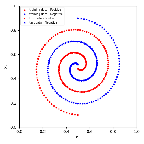
很显然, 此螺旋数据集并非线性可分.结果展示:
此局部加权模型在训练集与测试集上的正确率均达到100%.使用建议:
①. 权重参数$\tau$的获取极为关键, 很大程度上将影响模型的表达能力.
②. 泛化误差可能存在多个局部极值, 需要指定合适的范围, 再行采用黄金分割法进行搜索.参考文档:
螺旋数据集来源:https://www.cnblogs.com/tornadomeet/archive/2012/06/05/2537360.html

局部加权之逻辑回归(1) - Python实现