决策树与随机森林分类算法(Python实现),,一、原理:决策树:能
决策树与随机森林分类算法(Python实现),,一、原理:决策树:能
一、原理:
决策树:能够利用一些决策结点,使数据根据决策属性进行路径选择,达到分类的目的。
一般决策树常用于DFS配合剪枝,被用于处理一些单一算法问题,但也能进行分类。
也就是通过每一个结点的决策进行分类,那么关于如何设置这些结点的决策方式:
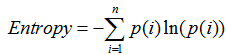
熵:描述一个集合内元素混乱程度的因素。
熵的衡量公式:
 ?
?
公式中的熵值Entropy会随着集合中类别数量增加而快速增加,也就是说一个集合中类别越少,那么它的熵就小,整体就越稳定。
对于一个标记数据集,要合理的建立一棵决策树,就需要合理的决定决策结点来使决策树尽快的降低熵值。
如何选择合适的决策:
(1)信息增溢
对于当前的集合,对每一个决策属性都尝试设置为决策结点的目标,计算决策分类前的熵值与分类后的所有子集的熵值的差。选择最大的,作为当前的决策目标。
此方式有一些确定,就是当面对一些决策变量的分类子集很多,而子集却很小的情况。这次办法虽然会很快的降低熵,但这并不是我们想要的。
(2)信息增溢率
这是对熵增溢的一种改进,把原本的前后熵值的差,增加:
决策分类前属性的熵和与决策分类后的的熵的比值,如果比值很小,说明分类分很多,损失值就会很大。
(3)gini系数:
gini系数和信息增溢率比较像
决策树的剪枝 :
预剪枝:设置max_depth来达到建树过程中的剪枝,表示树的最大深度
后剪枝:通过min_sample_split与min_sample_leaf来对已经建成的决策树进行剪枝,分别是结点的元素个数与子树的叶子结点个数
随机森林 :
构建多个决策树,从而得到更加符合期望的一些决策结果。以森林的结果众数来表示结果。
往往采用生成子数据集,取60%随机生成数据集
交叉验证:
几折交叉验证方式为,将训练数据进行几次对折,取一部分作为测试集,其他作为训练集。并将每个部分轮流作为测试集,最后得到一个平均评分。
网格超参数调优:
对分类器的参数进行调优评价,最后得到一个最优的参数组,并作为最终的分类器的参数。
二、实现 :
数据集:威斯康辛州乳腺癌数据集
import pandas as pddf = pd.read_csv(‘文件所在路径\\breast_cancer.csv‘,encoding=‘gbk‘)df.head()df.res.value_counts()y=df.resy.head()df=df.drop(index=0)#修正数据集x=df.drop(‘res‘,axis=1)#去掉标签
 ?
?
数据标签分布较为均衡
#导入决策树from sklearn.tree import DecisionTreeClassifier#导入随机森林from sklearn.ensemble import RandomForestClassifier#导入集合分割,交叉验证,网格搜索from sklearn.model_selection import train_test_split,cross_val_score,GridSearchCVseed=5#随机种子#分割训练集与测试集xtrain,xtest,ytrain,ytest=train_test_split(x,y,test_size=0.3,random_state=seed)#实例化随机森林rfc=RandomForestClassifier()#训练rfc=rfc.fit(xtrain,ytrain)测试评估result=rfc.score(xtest,ytest)
 ?
?
print(‘所有树:%s‘%rfc.estimators_)print(rfc.classes_)print(rfc.n_classes)print(‘判定结果:%s ‘%rfc.predict(xtest))print(‘判定结果:%s‘%rfc.predict_proba(xtest)[:,:])print(‘判定结果:%s ‘%rfc.predict_proba(xtest)[:,1])#d1与d2结果相同d1=np.array(pd.Series(rfc.predict_proba(xtest)[:,1]>0.5).map({False:0,True:1}))d2=rfc.predict(xtest)np.array_equal(d1,d2)#导入评价模块from sklearn.metrics import roc_auc_score,roc_curve,auc#准确率roc_auc_score(ytest,rfc.predict_proba(xtest)[:,1])#结果:0.9935171385991058print(‘各个feature的重要性:%s ‘%rfc.feature_importances_)std=np.std([tree.feature_importances_ for tree in rfc.estimators_],axis=0)从大到小排序indices = np.argsort(importances)[::-1]print(‘Feature Ranking:‘)for f in range(min(20,xtrain.shape[1])): print("%2d)%-*s %f"%(f+1, 30, xtrain.columns[indices[f]],importances[indices[f]])) ?
?
绘图#黑线是标准差plt.figure()plt.title("Feature importances")plt.bar(range(xtrain.shap[1]), importances[indices], color=‘r‘, yerr=std[indices], align="center")plt.xticks(range(xtrain.shap[1]), indices)plt.xlim([-1, xtrain.shap[1]])plt.show()predictions_validation = rfc.predict_proba(xtest)[:,1]fpr, tqr, _=roc_curve(ytest, predictions_validation)roc_auc = auc(fpr, tqr)plt.title(‘ROC Validation‘)plt.plot(fpr, tqr, ‘b‘, label=‘AUC = %0.2f‘%roc_auc)plt.legend(loc=‘lower right‘)plt.plot([0, 1], [0, 1], ‘r--‘)plt.xlim([0, 1])plt.ylim([0, 1])plt.ylabel(‘True Position Rate‘)plt.xlabel(‘False Postion Rate‘)plt.show() ?
?
 ?
?
‘‘‘交叉验证‘‘‘‘‘‘sklearn.model_selection.cross_val_score(estimator, X,yscoring=None, cv=None, n_jobs=1,verbose=0,fit_params=None,pre_dispatch=‘2*n_jobs‘)estimator:估计方法对象(分类器)X:数据特征(Featrues)y:数据标签(Labels)soring:调用方法(包括accuracy和mean_squared_error等等)cv:几折交叉验证(样本等分成几个部分,轮流作为验证集来验证模型)n_jobs:同时工作的cpu个数(-1 代表全部)‘‘‘#两种分类器的比较#决策树clf = DecisionTreeClassifier(max_depth=None,min_samples_split=2,random_state=0)scores = cross_val_score(clf, xtrain, ytrain)print(scores.mean())#0.932157394843962#随机森林clf = RandomForestClassifier()scores = cross_val_score(clf, xtrain, ytrain)print(scores.mean())#0.9471958389868838
参数调优过程:
#参数调优param_test1 = {‘n_estimators‘:range(25,500,25)}gsearch1 = GridSearchCV(estimator = RandomForestClassifier(min_samples_split=100, min_samples_leaf=20, max_depth=8,random_state=10), param_grid = param_test1, scoring=‘roc_auc‘, cv = 5)gsearch1.fit(xtrain, ytrain)‘‘‘调优结果‘‘‘print(gsearch1.best_params_,gsearch1.best_score_)param_test2 = {‘min_samples_split‘:range(60,200,20), ‘min_samples_leaf‘:range(10,110,10)}gsearch2 = GridSearchCV(estimator = RandomForestClassifier(n_estimators=50, max_depth=8,random_state=10), param_grid = param_test2, scoring=‘roc_auc‘, cv = 5)gsearch2.fit(xtrain, ytrain)‘‘‘调优结果‘‘‘print(gsearch2.best_params_,gsearch2.best_score_)param_test3 = {‘max_depth‘:range(3,30,2)}gsearch1 = GridSearchCV(estimator = RandomForestClassifier(min_samples_split=60, min_samples_leaf=10, n_estimators=50, random_state=10), param_grid = param_test3, scoring=‘roc_auc‘, cv = 5)gsearch3.fit(xtrain, ytrain)‘‘‘调优结果‘‘‘print(gsearch3.best_params_,gsearch3.best_score_)param_test4 = {‘criterion‘:[‘gini‘,‘entropy‘], ‘class_weight‘:[None, ‘balanced‘]}gsearch4 = GridSearchCV(estimator = RandomForestClassifier(n_estimators=50, min_samples_split=60, min_samples_leaf=10, max_depth=3, random_state=10), param_grid = param_test4, scoring=‘roc_auc‘, cv = 5)gsearch4.fit(xtrain, ytrain)‘‘‘调优结果‘‘‘print(gsearch4.best_params_,gsearch4.best_score_)#gini,None#整合所有最优参数值,得到最优评分best_score = roc_auc_score(ytest, gsearch4.best_estimator_.predict_proba(xtest)[:,1])print(best_score)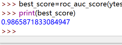 ?
?
决策树与随机森林分类算法(Python实现)
相关内容
- python 爬取百度图片,百度图片识别,import req
- 怎么手动安装python 官方whl包、tar.gz包、zip包,python压缩
- Python 东方财富网-股市行情数据抓取,,东方财富网 股市
- python + selenium + unittest 自动化测试框架 -- 入门篇,
- PyCharm+cmd中使用Anaconda 与 新建Python环境(Windows),,P
- Python 5行代码 搞定加减法计算,加减法速算口诀,五行代
- python接口测试-自动化测试报告生成。,,1. 首先创建r
- Python接口自动化之登录接口测试,,在上一篇Python
- Python爬取51job职位信息,,# -*- codi
- Python3 upper()方法,python中lower什么意思,描述Python u
评论关闭