《Python机器学习时间指南》一、Python机器学习的生态系统，,　　本文主要记录《P

《Python机器学习时间指南》一、Python机器学习的生态系统，,　　本文主要记录《P

　　本文主要记录《Python机器学习时间指南》第一章中1.2Python库和功能中的内容。学习机器学习的工作流程。

一、数据的获取和检查

requests获取数据

pandans处理数据

 1 import os 2 import pandas as pd 3 import requests 4  5 PATH = r‘E:/Python Machine Learning Blueprints/Chap1/1.2/‘ 6 r = requests.get(‘https://archive.ics.uci.edu/ml/machine-learning-databases/iris/iris.data‘) 7 with open(PATH + ‘iris.data‘, ‘w‘) as f: 8          f.write(r.text) 9 os.chdir(PATH)10 df = pd.read_csv(PATH + ‘iris.data‘, names=[‘sepal length‘,‘sepal width‘,‘petal length‘,‘petal width‘,‘class‘])11 df.head()

注意：1、requests库为访问数据的API交互借口，pandas是数据分析工具，两者可以专门拿出来后续研究

2、read_csv后的路径名不能含有中文，否则会报OSError: Initializing from file failed。

上述程序运行结果：

sepal length sepal width petal length petal width class
0 5.1 3.5 1.4 0.2 Iris-setosa
1 4.9 3.0 1.4 0.2 Iris-setosa
2 4.7 3.2 1.3 0.2 Iris-setosa
3 4.6 3.1 1.5 0.2 Iris-setosa
4 5.0 3.6 1.4 0.2 Iris-setosa
5 5.4 3.9 1.7 0.4 Iris-setosa
6 4.6 3.4 1.4 0.3 Iris-setosa
7 5.0 3.4 1.5 0.2 Iris-setosa...

书中对于df的处理中值得注意的操作：

（1）过滤：

df[(df[‘class‘] == ‘Iris-setosa‘)&(df[‘petal width‘]>2.2)]

sepal length sepal width petal length petal width class
100 6.3 3.3 6.0 2.5 Iris-virginica
109 7.2 3.6 6.1 2.5 Iris-virginica
114 5.8 2.8 5.1 2.4 Iris-virginica
115 6.4 3.2 5.3 2.3 Iris-virginica
118 7.7 2.6 6.9 2.3 Iris-virginica
120 6.9 3.2 5.7 2.3 Iris-virginica
135 7.7 3.0 6.1 2.3 Iris-virginica
136 6.3 3.4 5.6 2.4 Iris-virginica
140 6.7 3.1 5.6 2.4 Iris-virginica
141 6.9 3.1 5.1 2.3 Iris-virginica
143 6.8 3.2 5.9 2.3 Iris-virginica
144 6.7 3.3 5.7 2.5 Iris-virginica
145 6.7 3.0 5.2 2.3 Iris-virginica
148 6.2 3.4 5.4 2.3 Iris-virginica

（2）过滤出的数据重新保存并重置索引

virginicadf = df[(df[‘class‘] == ‘Iris-virginica‘)&(df[‘petal width‘]>2.2)].reset_index(drop=True)

（3）获得各列统计信息

df.describe()

（4）每行-列相关系数

df.corr()

matplotlib绘制数据

（1）条形图（hist）

 1 import matplotlib.pyplot as plt 2 plt.style.use(‘ggplot‘) 3 #%matplotlib inline 4 import numpy as np 5  6 fig,ax = plt.subplots(figsize=(6,4)) 7 ax.hist(df[‘petal width‘], color=‘black‘) 8 ax.set_ylabel(‘Count‘,fontsize=12) 9 ax.set_xlabel(‘Width‘,fontsize=12)10 plt.title(‘Iris Petal Width‘,fontsize=14, y=1.01)11 plt.show()

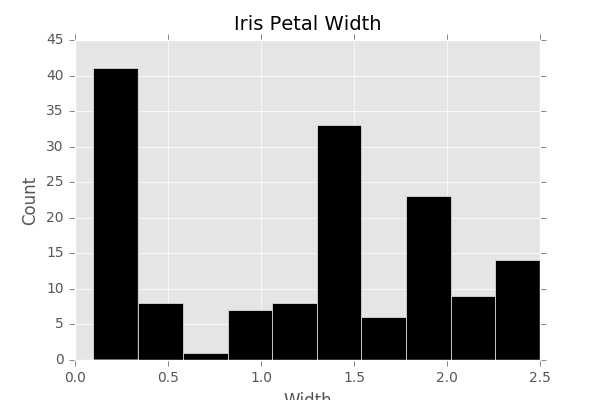
注意：%matplotlib inline为ipython中语句，先暂时封掉；figsize=(6,4)不要漏掉=。为了显示，在最后加了show()函数

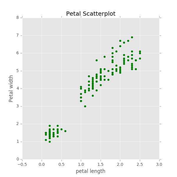
（2）散点图（scatter）

1 fig,ax = plt.subplots(figsize=(6,6))2 ax.scatter(df[‘petal width‘],df[‘petal length‘], color=‘green‘)3 ax.set_ylabel(‘Petal width‘,fontsize=12)4 ax.set_xlabel(‘petal length‘,fontsize=12)5 plt.title(‘Petal Scatterplot‘)6 plt.show()

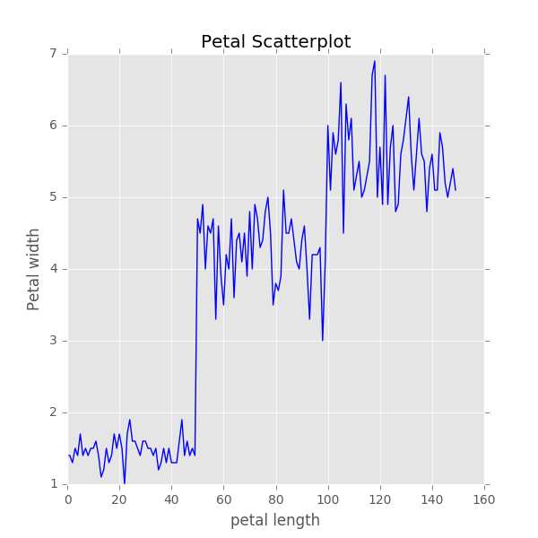
（3）直接绘制折线图（plot）

1 fig,ax = plt.subplots(figsize=(6,6))2 ax.scatter(df[‘petal width‘],df[‘petal length‘], color=‘green‘)3 ax.set_ylabel(‘Petal width‘,fontsize=12)4 ax.set_xlabel(‘petal length‘,fontsize=12)5 plt.title(‘Petal Scatterplot‘)6 plt.show()

（4）堆积条形图

 1 fig,ax = plt.subplots(figsize=(6,6)) 2 bar_width = .8 3 labels = [x for x in df.columns if ‘length‘ in x or ‘width‘ in x] 4 ver_y = [df[df[‘class‘]==‘Iris-versicolor‘][x].mean() for x in labels] 5 vir_y = [df[df[‘class‘]==‘Iris-virginica‘][x].mean() for x in labels] 6 set_y = [df[df[‘class‘]==‘Iris-setosa‘][x].mean() for x in labels] 7 x = np.arange(len(labels)) 8 ax.bar(x,vir_y,bar_width,bottom=set_y,color=‘darkgrey‘) 9 ax.bar(x,set_y,bar_width,bottom=ver_y,color=‘white‘)10 ax.bar(x,ver_y,bar_width,color=‘black‘)11 ax.set_xticks(x+(bar_width/2))12 ax.set_xticklabels(labels,rotation=-70,fontsize=12)13 ax.set_title(‘Mean Feature Measurement By Class‘,y=1.01)14 ax.legend([‘Virginica‘,‘Setosa‘,‘Versicolor‘])

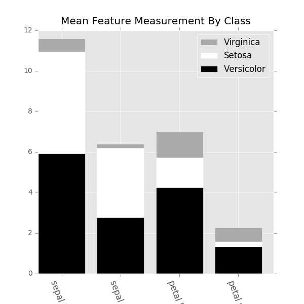
注意：8-10行的代码是按照三种类型从高到低排的，如果调换了顺序结果错误。

Seaborn库统计可视化

利用Seaborn库可以简单获取数据的相关性和特征。

二、准备

1、Map

df[‘class‘] = df[‘class‘].map({‘Iris-setosa‘:‘SET‘,‘Iris-virginica‘:‘VIR‘,‘Iris-versicolor‘:‘VER‘})

sepal length sepal width petal length petal width class
0 5.1 3.5 1.4 0.2 SET
1 4.9 3.0 1.4 0.2 SET
2 4.7 3.2 1.3 0.2 SET
3 4.6 3.1 1.5 0.2 SET
4 5.0 3.6 1.4 0.2 SET
5 5.4 3.9 1.7 0.4 SET
6 4.6 3.4 1.4 0.3 SET

2、Apply对行或列操作

应用在某一列：df[‘width petal‘] = df[‘petal width‘].apply(lambda v: 1 if v >=1.3 else 0)

在df中添加一列width petal 如果petal width超过1.3则为1，否则为0。注意lambda v是df[‘petal width‘]的返回值

应用在数据框：df[‘width area‘]=df.apply[lambda r: r[‘petal length‘] * r[‘petal width‘], axis=1]

注：axis=1表示对行运用函数，axis=0表示对列应用函数。所以上面的lambda r返回的是每一行

3、ApplyMap对所有单元执行操作

df.applymap(lambda v: np.log(v) if isinstance(v,float) else v)

4、Groupby 基于某些选择的列别对数据进行分组

df.groupby(‘class‘).mean()

数据按class分类并分别给出平均值

sepal length sepal width petal length petal width
class
Iris-setosa 5.006 3.418 1.464 0.244
Iris-versicolor 5.936 2.770 4.260 1.326
Iris-virginica 6.588 2.974 5.552 2.026

df.groupby(‘class‘).describe()

数据按class分裂并分别给出描述统计信息

petal length \
count mean std min 25% 50% 75% max
class
Iris-setosa 50.0 1.464 0.173511 1.0 1.4 1.50 1.575 1.9
Iris-versicolor 50.0 4.260 0.469911 3.0 4.0 4.35 4.600 5.1
Iris-virginica 50.0 5.552 0.551895 4.5 5.1 5.55 5.875 6.9

petal width ... sepal length sepal width \
count mean ... 75% max count mean
class ...
Iris-setosa 50.0 0.244 ... 5.2 5.8 50.0 3.418
Iris-versicolor 50.0 1.326 ... 6.3 7.0 50.0 2.770
Iris-virginica 50.0 2.026 ... 6.9 7.9 50.0 2.974

std min 25% 50% 75% max
class
Iris-setosa 0.381024 2.3 3.125 3.4 3.675 4.4
Iris-versicolor 0.313798 2.0 2.525 2.8 3.000 3.4
Iris-virginica 0.322497 2.2 2.800 3.0 3.175 3.8

df.groupby(‘class‘)[‘petal width‘].agg({‘delta‘:lambda x:x.max()-x.min(), ‘max‘:np.max, ‘min‘:np.min})

delta max min
class
Iris-setosa 0.5 0.6 0.1
Iris-versicolor 0.8 1.8 1.0
Iris-virginica 1.1 2.5 1.4

三、建模和评估

这里只是简单运用两个函数，详细的内容见后面的内容

注：本章涉及到的可以详细了解的库：

requests、pandans、matplotlib、seaborn、statsmodels、scikit-learn

《Python机器学习时间指南》一、Python机器学习的生态系统