用Python实现文档聚类，,未经许可，禁止转载！英文

用Python实现文档聚类，,未经许可，禁止转载！英文

本文由 编橙之家 - Ree Ray 翻译，LynnShaw 校稿。未经许可，禁止转载！
英文出处：brandonrose。欢迎加入翻译组。

在本教程中，我会利用 Python 来说明怎样聚类一系列的文档。我所演示的实例会识别出 top 100 电影的（来自 IMDB 列表）剧情简介的隐藏结构。关于这个例子的详细讨论在初始版本里。本教程包括：

• 对所有剧情简介分词（tokenizing）和词干化（stemming）
• 利用 tf-idf 将语料库转换为向量空间（vector space）
• 计算每个文档间的余弦距离（cosine distance）用以测量相似度
• 利用 k-means 算法进行文档聚类
• 利用多维尺度分析（multidimensional scaling）对语料库降维
• 利用 matplotlib 和 mpld3 绘制输出的聚类
• 对语料库进行Ward 聚类算法生成层次聚类（hierarchical clustering）
• 绘制 Ward 树状图（Ward dendrogram）
• 利用 隐含狄利克雷分布（LDA） 进行主题建模

整个项目在我的 github repo 都可以找到。其中‘cluster_analysis ‘工作簿是一个完整的版本；‘cluster_analysis_web’ 为了创建教程则经过了删减。欢迎下载代码并使用‘cluster_analysis’ 进行单步调试（step through）。

如果你有任何问题，欢迎用推特来联系我 @brandonmrose。

在此之前，我先在前面导入所有需要用到的库

Python

import numpy as np
import pandas as pd
import nltk
import re
import os
import codecs
from sklearn import feature_extraction
import mpld3

出于走查的目的，想象一下我有 2 个主要的列表：

• ‘titles’：按照排名的影片名称
• ‘synopses’：对应片名列表的剧情简介

我在 github 上 po 出来的完整工作簿已经导入了上述列表，但是为了简洁起见，我会直接使用它们。其中最最重要的是 ‘synopses’ 列表了，‘titles’ 更多是作为了标记用的。

Python

print titles[:10] #前 10 个片名

Python

['The Godfather', 'The Shawshank Redemption', "Schindler's List", 'Raging Bull', 'Casablanca', "One Flew Over the Cuckoo's Nest", 'Gone with the Wind', 'Citizen Kane', 'The Wizard of Oz', 'Titanic']

停用词，词干化与分词

本节我将会定义一些函数对剧情简介进行处理。首先，我载入 NLTK 的英文停用词列表。停用词是类似“a”，“the”，或者“in”这些无法传达重要意义的词。我相信除此之外还有更好的解释。

Python

# 载入 nltk 的英文停用词作为“stopwords”变量
stopwords = nltk.corpus.stopwords.words('english')

Python

print stopwords[:10]

Python

['i', 'me', 'my', 'myself', 'we', 'our', 'ours', 'ourselves', 'you', 'your']

接下来我导入 NLTK 中的 Snowball 词干分析器（Stemmer）。词干化（Stemming）的过程就是将词打回原形。

Python

# 载入 nltk 的 SnowballStemmer 作为“stemmer”变量
from nltk.stem.snowball import SnowballStemmer
stemmer = SnowballStemmer("english")

以下我定义了两个函数：

• tokenize_and_stem：对每个词例（token）分词（tokenizes）（将剧情简介分割成单独的词或词例列表）并词干化
• tokenize_only: 分词即可

我利用上述两个函数创建了一个重要的字典，以防我在后续算法中需要使用词干化后的词（stems）。出于展示的目的，后面我又会将这些词转换回它们原本的的形式。猜猜看会怎样，我实在想试试看！

Python

# 这里我定义了一个分词器（tokenizer）和词干分析器（stemmer），它们会输出给定文本词干化后的词集合

def tokenize_and_stem(text):
    # 首先分句，接着分词，而标点也会作为词例存在
    tokens = [word for sent in nltk.sent_tokenize(text) for word in nltk.word_tokenize(sent)]
    filtered_tokens = []
    # 过滤所有不含字母的词例（例如：数字、纯标点）
    for token in tokens:
        if re.search('[a-zA-Z]', token):
            filtered_tokens.append(token)
    stems = [stemmer.stem(t) for t in filtered_tokens]
    return stems


def tokenize_only(text):
    # 首先分句，接着分词，而标点也会作为词例存在
    tokens = [word.lower() for sent in nltk.sent_tokenize(text) for word in nltk.word_tokenize(sent)]
    filtered_tokens = []
    # 过滤所有不含字母的词例（例如：数字、纯标点）
    for token in tokens:
        if re.search('[a-zA-Z]', token):
            filtered_tokens.append(token)
    return filtered_tokens

接下来我会使用上述词干化/分词和分词函数遍历剧情简介列表以生成两个词汇表：经过词干化和仅仅经过分词后。

Python

# 非常不 pythonic，一点也不！
# 扩充列表后变成了非常庞大的二维（flat）词汇表
totalvocab_stemmed = []
totalvocab_tokenized = []
for i in synopses:
    allwords_stemmed = tokenize_and_stem(i) #对每个电影的剧情简介进行分词和词干化
    totalvocab_stemmed.extend(allwords_stemmed) # 扩充“totalvocab_stemmed”列表

    allwords_tokenized = tokenize_only(i)
    totalvocab_tokenized.extend(allwords_tokenized)

利用上述两个列表，我创建了一个 pandas 的 DataFrame，以词干化后的词汇表作为索引，分词后的词为列。这么做便于观察词干化后的词转换回完整的词例。以下展示词干化后的词变回原词例是一对多（one to many）的过程：词干化后的“run”能够关联到“ran”，“runs”，“running”等等。在我看来这很棒——我非常愿意将我需要观察的词干化过后的词转换回第一个联想到的词例。

Python

vocab_frame = pd.DataFrame({'words': totalvocab_tokenized}, index = totalvocab_stemmed)
print 'there are ' + str(vocab_frame.shape[0]) + ' items in vocab_frame'

Python

there are 312209 items in vocab_frame

你会注意到有些重复的地方。我可以把它清理掉，不过鉴于 DataFrame 只有 312209 项，并不是很庞大，可以用 stem-index 来观察词干化后的词。

Python

print vocab_frame.head()

Python

words
plot  plot
edit  edit
edit  edit
edit  edit
on      on

Tf-idf 与文本相似度

下面，我定义词频-逆向文件频率（tf-idf）的向量化参数，把剧情简介列表都转换成 tf-idf 矩阵。

为了得到 TF-IDF 矩阵，首先计算词在文档中的出现频率，它会被转换成文档-词矩阵（dtm），也叫做词频（term frequency）矩阵。dtm 的例子如下图所示：

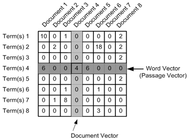
接着使用 TF-IDF 权重：某些词在某个文档中出现频率高，在其他文中却不常出现，那么这些词具有更高的 TF-IDF 权重，因为这些词被认为在相关文档中携带更多信息。

注意我下面定义的几个参数：

• max_df：这个给定特征可以应用在 tf-idf 矩阵中，用以描述单词在文档中的最高出现率。假设一个词（term）在 80% 的文档中都出现过了，那它也许（在剧情简介的语境里）只携带非常少信息。
• min_df：可以是一个整数（例如5）。意味着单词必须在 5 个以上的文档中出现才会被纳入考虑。在这里我设置为 0.2；即单词至少在 20% 的文档中出现 。因为我发现如果我设置更小的 min_df，最终会得到基于姓名的聚类（clustering）——举个例子，好几部电影的简介剧情中老出现“Michael”或者“Tom”这些名字，然而它们却不携带什么真实意义。
• ngram_range：这个参数将用来观察一元模型（unigrams），二元模型（ bigrams） 和三元模型（trigrams）。参考n元模型（n-grams）。

Python

from sklearn.feature_extraction.text import TfidfVectorizer

# 定义向量化参数
tfidf_vectorizer = TfidfVectorizer(max_df=0.8, max_features=200000,
                                 min_df=0.2, stop_words='english',
                                 use_idf=True, tokenizer=tokenize_and_stem, ngram_range=(1,3))

%time tfidf_matrix = tfidf_vectorizer.fit_transform(synopses) # 向量化剧情简介文本

print(tfidf_matrix.shape)

Python

CPU times: user 29.1 s, sys: 468 ms, total: 29.6 s
Wall time: 37.8 s
(100, 563)

“terms” 这个变量只是 tf-idf 矩阵中的特征（features）表，也是一个词汇表。

Python

terms = tfidf_vectorizer.get_feature_names()

dist 变量被定义为 1 – 每个文档的余弦相似度。余弦相似度用以和 tf-idf 相互参照评价。可以评价全文（剧情简介）中文档与文档间的相似度。被 1 减去是为了确保我稍后能在欧氏（euclidean）平面（二维平面）中绘制余弦距离。

注意 dist 可以用以评估任意两个或多个剧情简介间的相似度。

Python

from sklearn.metrics.pairwise import cosine_similarity
dist = 1 - cosine_similarity(tfidf_matrix)

K-means 聚类

下面开始好玩的部分。利用 tf-idf 矩阵，你可以跑一长串聚类算法来更好地理解剧情简介集里的隐藏结构。我首先用 k-means 算法。这个算法需要先设定聚类的数目（我设定为 5）。每个观测对象（observation）都会被分配到一个聚类，这也叫做聚类分配（cluster assignment）。这样做是为了使组内平方和最小。接下来，聚类过的对象通过计算来确定新的聚类质心（centroid）。然后，对象将被重新分配到聚类，在下一次迭代操作中质心也会被重新计算，直到算法收敛。

跑了几次这个算法以后我发现得到全局最优解（global optimum）的几率要比局部最优解（local optimum）大。

Python

from sklearn.cluster import KMeans

num_clusters = 5

km = KMeans(n_clusters=num_clusters)

%time km.fit(tfidf_matrix)

clusters = km.labels_.tolist()

Python

CPU times: user 232 ms, sys: 6.64 ms, total: 239 ms
Wall time: 305 ms

利用 joblib.dump pickle 模型（model），一旦算法收敛，重载模型并分配聚类标签（labels）。

Python

from sklearn.externals import joblib

# 注释语句用来存储你的模型
# 因为我已经从 pickle 载入过模型了

#joblib.dump(km,  'doc_cluster.pkl')

km = joblib.load('doc_cluster.pkl')
clusters = km.labels_.tolist()

下面，我创建了一个字典，包含片名，排名，简要剧情，聚类分配，还有电影类型（genre）（排名和类型是从 IMDB 上爬下来的）。

为了方便起见，我将这个字典转换成了 Pandas DataFrame。我是 Pandas 的脑残粉，我强烈建议你了解一下它惊艳的功能。这些我下面就会使用到，但不会深入。

Python

films = { 'title': titles, 'rank': ranks, 'synopsis': synopses, 'cluster': clusters, 'genre': genres }

frame = pd.DataFrame(films, index = [clusters] , columns = ['rank', 'title', 'cluster', 'genre'])

Python

frame['cluster'].value_counts() #number of films per cluster (clusters from 0 to 4)

Python

4 26

Python

0    25
2    21
1    16
3    12
dtype: int64

Python

grouped = frame['rank'].groupby(frame['cluster']) # 为了凝聚（aggregation），由聚类分类。

grouped.mean() # 每个聚类的平均排名（1 到 100）

Python

cluster
0          47.200000
1          58.875000
2          49.380952
3          54.500000
4          43.730769
dtype: float64

clusters 4 和 clusters 0 的排名最低，说明它们包含的影片在 top 100 列表中相对没那么棒。

在这选取 n（我选 6 个） 个离聚类质心最近的词对聚类进行一些好玩的索引（indexing）和排列（sorting）。这样可以更直观观察聚类的主要主题。

Python

from __future__ import print_function

print("Top terms per cluster:")
print()
# 按离质心的距离排列聚类中心，由近到远
order_centroids = km.cluster_centers_.argsort()[:, ::-1] 

for i in range(num_clusters):
    print("Cluster %d words:" % i, end='')

    for ind in order_centroids[i, :6]: # 每个聚类选 6 个词
        print(' %s' % vocab_frame.ix[terms[ind].split(' ')].values.tolist()[0][0].encode('utf-8', 'ignore'), end=',')
    print() # 空行
    print() # 空行

    print("Cluster %d titles:" % i, end='')
    for title in frame.ix[i]['title'].values.tolist():
        print(' %s,' % title, end='')
    print() # 空行
    print() # 空行

聚类中的前几项：

聚类 0 中的单词: family, home, mother, war, house, dies,

聚类 0 中的片名: Schindler’s List, One Flew Over the Cuckoo’s Nest, Gone with the Wind, The Wizard of Oz, Titanic, Forrest Gump, E.T. the Extra-Terrestrial, The Silence of the Lambs, Gandhi, A Streetcar Named Desire, The Best Years of Our Lives, My Fair Lady, Ben-Hur, Doctor Zhivago, The Pianist, The Exorcist, Out of Africa, Good Will Hunting, Terms of Endearment, Giant, The Grapes of Wrath, Close Encounters of the Third Kind, The Graduate, Stagecoach, Wuthering Heights,

聚类 1 中的单词: police, car, killed, murders, driving, house,

聚类 1 中的片名: Casablanca, Psycho, Sunset Blvd., Vertigo, Chinatown, Amadeus, High Noon, The French Connection, Fargo, Pulp Fiction, The Maltese Falcon, A Clockwork Orange, Double Indemnity, Rebel Without a Cause, The Third Man, North by Northwest,

聚类 2 中的单词: father, new, york, new, brothers, apartments,

聚类 2 中的片名: The Godfather, Raging Bull, Citizen Kane, The Godfather: Part II, On the Waterfront, 12 Angry Men, Rocky, To Kill a Mockingbird, Braveheart, The Good, the Bad and the Ugly, The Apartment, Goodfellas, City Lights, It Happened One Night, Midnight Cowboy, Mr. Smith Goes to Washington, Rain Man, Annie Hall, Network, Taxi Driver, Rear Window,

聚类 3 中的单词: george, dance, singing, john, love, perform,

聚类 3 中的片名: West Side Story, Singin’ in the Rain, It’s a Wonderful Life, Some Like It Hot, The Philadelphia Story, An American in Paris, The King’s Speech, A Place in the Sun, Tootsie, Nashville, American Graffiti, Yankee Doodle Dandy,

聚类 4 中的单词: killed, soldiers, captain, men, army, command,

聚类 4 中的片名: The Shawshank Redemption, Lawrence of Arabia, The Sound of Music, Star Wars, 2001: A Space Odyssey, The Bridge on the River Kwai, Dr. Strangelove or: How I Learned to Stop Worrying and Love the Bomb, Apocalypse Now, The Lord of the Rings: The Return of the King, Gladiator, From Here to Eternity, Saving Private Ryan, Unforgiven, Raiders of the Lost Ark, Patton, Jaws, Butch Cassidy and the Sundance Kid, The Treasure of the Sierra Madre, Platoon, Dances with Wolves, The Deer Hunter, All Quiet on the Western Front, Shane, The Green Mile, The African Queen, Mutiny on the Bounty,

多维尺度分析（Multidimensional scaling）

利用下面多维尺度分析（MDS）的代码将距离矩阵转化为一个二维数组。我并不想假装我很了解MDS，不过这个算法很管用。另外可以用 特征降维（principal component analysis） 来完成这个任务。

Python

import os  # 为了使用 os.path.basename 函数

import matplotlib.pyplot as plt
import matplotlib as mpl

from sklearn.manifold import MDS

MDS()

# 将二位平面中绘制的点转化成两个元素（components）
# 设置为“precomputed”是因为我们提供的是距离矩阵
# 我们可以将“random_state”具体化来达到重复绘图的目的
mds = MDS(n_components=2, dissimilarity="precomputed", random_state=1)

pos = mds.fit_transform(dist)  # 形如 (n_components, n_samples)

xs, ys = pos[:, 0], pos[:, 1]

可视化文档聚类

本节中，我会演示怎样利用 matplotlib 和 mpld3（将 matplotlib 封装成 D3.js）来实现文档聚类的可视化。

首先，我定义了一些字典，让聚类的编号和聚类绘色，聚类名称一一对应。其中聚类对应的名称是从离聚类质心最近的单词中挑选出来的。

Python

# 用字典设置每个聚类的颜色
cluster_colors = {0: '#1b9e77', 1: '#d95f02', 2: '#7570b3', 3: '#e7298a', 4: '#66a61e'}

# 用字典设置每个聚类名称
cluster_names = {0: 'Family, home, war', 
                 1: 'Police, killed, murders', 
                 2: 'Father, New York, brothers', 
                 3: 'Dance, singing, love', 
                 4: 'Killed, soldiers, captain'}

下面我会用 matplotlib 来绘制彩色的带标签的观测对象（影片，片名）。关于 matplotlib 绘图我不想讨论太多，但我尽可能提供一些有用的注释。

Python

# 在 ipython 中内联（inline）演示 matplotlib 绘图
%matplotlib inline 

# 用 MDS 后的结果加上聚类编号和绘色创建 DataFrame
df = pd.DataFrame(dict(x=xs, y=ys, label=clusters, title=titles)) 

# 聚类归类
groups = df.groupby('label')


# 设置绘图
fig, ax = plt.subplots(figsize=(17, 9)) # 设置大小
ax.margins(0.05) # 可选项，只添加 5% 的填充（padding）来自动缩放（auto scaling）。

# 对聚类进行迭代并分布在绘图上
# 我用到了 cluster_name 和 cluster_color 字典的“name”项，这样会返回相应的 color 和 label
for name, group in groups:
    ax.plot(group.x, group.y, marker='o', linestyle='', ms=12, 
            label=cluster_names[name], color=cluster_colors[name], 
            mec='none')
    ax.set_aspect('auto')
    ax.tick_params(
        axis= 'x',          # 使用 x 坐标轴
        which='both',      # 同时使用主刻度标签（major ticks）和次刻度标签（minor ticks）
        bottom='off',      # 取消底部边缘（bottom edge）标签
        top='off',         # 取消顶部边缘（top edge）标签
        labelbottom='off')
    ax.tick_params(
        axis= 'y',         # 使用 y 坐标轴
        which='both',      # 同时使用主刻度标签（major ticks）和次刻度标签（minor ticks）
        left='off',      # 取消底部边缘（bottom edge）标签
        top='off',         # 取消顶部边缘（top edge）标签
        labelleft='off')

ax.legend(numpoints=1)  # 图例（legend）中每项只显示一个点

# 在坐标点为 x,y 处添加影片名作为标签（label）
for i in range(len(df)):
    ax.text(df.ix[i]['x'], df.ix[i]['y'], df.ix[i]['title'], size=8)  



plt.show() # 展示绘图

# 以下注释语句可以保存需要的绘图
#plt.savefig('clusters_small_noaxes.png', dpi=200)

Python

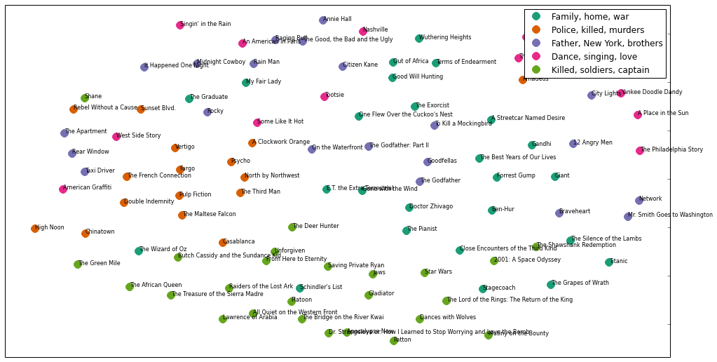
plt.close()

绘制的聚类分布图看起来不错，但是重叠在一起的标签真是亮瞎了眼。因为之前使用过 D3.js，所以我知道有个解决方案是基于浏览器和 javascript 交互的。所幸我最近偶然发现了 mpld3，是基于 matplotlib 的 D3 封装。Mpld3 主要可以让你使用 matplotlib 的语法实现网页交互。它非常容易上手，当你遇到感兴趣的内容，鼠标停驻的时候，利用高效的接口可以添加气泡提示。

另外，它还提供了缩放和拖动这么炫的功能。以下的 javascript 片段主要自定义了缩放和拖动的位置。别太担心，实际上你用不到它，但是稍后导出到网页的时候有利于格式化。你唯一想要改变的应该是借助 x 和 y 的 attr 来改变工具栏的位置。

Python

# 自定义工具栏（toolbar）位置
class TopToolbar(mpld3.plugins.PluginBase):
    """移动工具栏到分布图顶部的插件"""

    JAVASCRIPT = """
    mpld3.register_plugin("toptoolbar", TopToolbar);
    TopToolbar.prototype = Object.create(mpld3.Plugin.prototype);
    TopToolbar.prototype.constructor = TopToolbar;
    function TopToolbar(fig, props){
        mpld3.Plugin.call(this, fig, props);
    };

    TopToolbar.prototype.draw = function(){
      //  还缺少工具栏 svg，因此一开始要绘制
      this.fig.toolbar.draw();

      // 接着把 y 的位置变为图顶部
      this.fig.toolbar.toolbar.attr("x", 150);
      this.fig.toolbar.toolbar.attr("y", 400);

      // 再移除 draw 函数，防止被调用
      this.fig.toolbar.draw = function() {}
    }
    """
    def __init__(self):
        self.dict_ = {"type": "toptoolbar"}

下面是对于交互式散点图的实际操作。我同样不会深入这个问题因为是直接从 mpld3 的例程移植过来的。虽然我用 pandas 对聚类进行了归类，但它们一一迭代后会分布在散点图上。和原生 D3 相比，用 mpld3 来做这项工作并且嵌入到 python 的工作簿中简单多了。如果你看了我网站上的其它内容，你就知道我有多么爱 D3 了。但以后一些基本的交互我可能还是会用 mpld3。

记住 mpld3 还可以自定义 CSS，像我设计的字体，坐标轴还有散点图左边的间距（margin）。

Python

# 用 MDS 后的结果加上聚类编号和绘色创建 DataFrame
df = pd.DataFrame(dict(x=xs, y=ys, label=clusters, title=titles)) 

# 聚类归类
groups = df.groupby('label')

# 自定义 css 对字体格式化以及移除坐标轴标签
css = """
text.mpld3-text, div.mpld3-tooltip {
  font-family:Arial, Helvetica, sans-serif;
}

g.mpld3-xaxis, g.mpld3-yaxis {
display: none; }

svg.mpld3-figure {
margin-left: -200px;}
"""

# 绘图 
fig, ax = plt.subplots(figsize=(14,6)) # 设置大小
ax.margins(0.03) # 可选项，只添加 5% 的填充（padding）来自动缩放

# 对聚类进行迭代并分布在绘图上
# 我用到了 cluster_name 和 cluster_color 字典的“name”项，这样会返回相应的 color 和 label
for name, group in groups:
    points = ax.plot(group.x, group.y, marker='o', linestyle='', ms=18, 
                     label=cluster_names[name], mec='none', 
                     color=cluster_colors[name])
    ax.set_aspect('auto')
    labels = [i for i in group.title]

    # 用点来设置气泡消息，标签以及已经定义的“css”
    tooltip = mpld3.plugins.PointHTMLTooltip(points[0], labels,
                                       voffset=10, hoffset=10, css=css)
    # 将气泡消息与散点图联系起来
    mpld3.plugins.connect(fig, tooltip, TopToolbar())    

    # 隐藏刻度线（tick marks）
    ax.axes.get_xaxis().set_ticks([])
    ax.axes.get_yaxis().set_ticks([])

    # 隐藏坐标轴
    ax.axes.get_xaxis().set_visible(False)
    ax.axes.get_yaxis().set_visible(False)


ax.legend(numpoints=1) # 图例中每项只显示一个点

mpld3.display() # 展示绘图

# 以下注释语句可以输出 html
#html = mpld3.fig_to_html(fig)
#print(html)

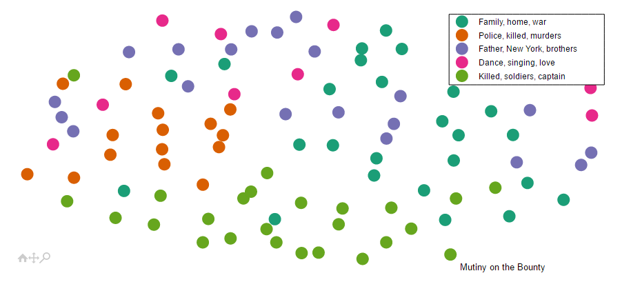
（译者按：因为无法插入 js，所以对原 post 截图）

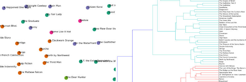
文档层次聚类

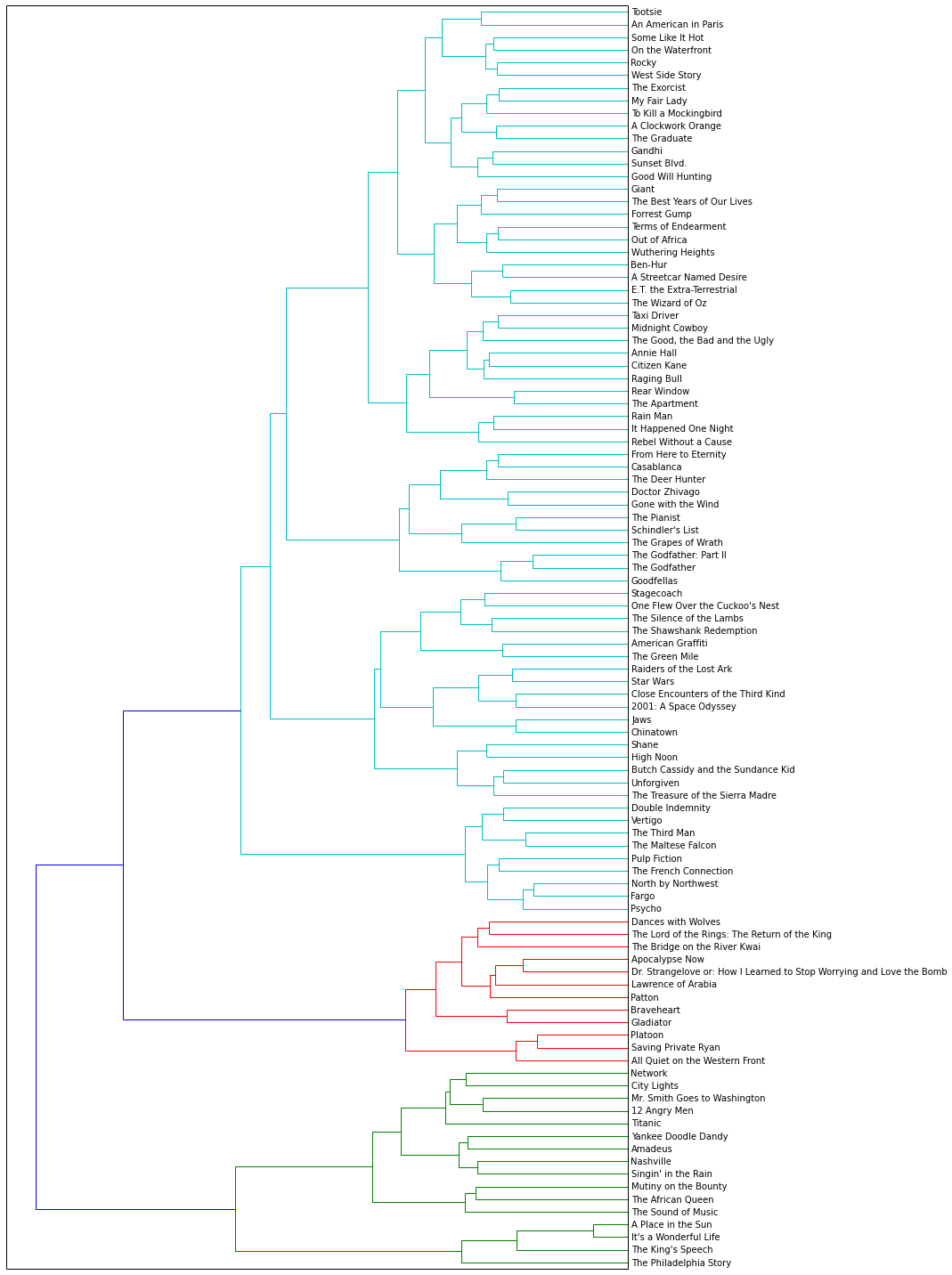
到目前为止我已经成功用 k-means 算法将文档聚类并绘制了结果，下面我想尝试其它聚类算法。我选择了 Ward 聚类算法 ，因为它可以进行层次聚类。Ward 聚类属于凝聚（agglomerative）聚类算法，亦即在每个处理阶段，聚类间两点距离最小的会被合并成一个聚类。我用之前计算得到的余弦距离矩阵（dist）来计算 linkage_matrix，等会我会把它绘制在树状图中。

值得注意的是这个算法返回了 3 组主要的聚类，最大聚类又被分成了 4 个主要的子聚类。其中红色标注的聚类包含了多部“Killed, soldiers, captain”主题下的影片。Braveheart 和 Gladiator* 是我最喜欢的两部片子，它们都在低层（low-level）的聚类里。

Python

from scipy.cluster.hierarchy import ward, dendrogram

linkage_matrix = ward(dist) # 聚类算法处理之前计算得到的距离，用 linkage_matrix 表示

fig, ax = plt.subplots(figsize=(15, 20)) # 设置大小
ax = dendrogram(linkage_matrix, orientation="right", labels=titles);

plt.tick_params(
        axis= 'x',          # 使用 x 坐标轴
        which='both',      # 同时使用主刻度标签（major ticks）和次刻度标签（minor ticks）
        bottom='off',      # 取消底部边缘（bottom edge）标签
        top='off',         # 取消顶部边缘（top edge）标签
    labelbottom='off')

plt.tight_layout() # 展示紧凑的绘图布局

# 注释语句用来保存图片
plt.savefig('ward_clusters.png', dpi=200) # 保存图片为 ward_clusters

Python

plt.close()

隐含狄利克雷分布

本节的重点放在如何利用 隐含狄利克雷分布（LDA）发掘 top 100 影片剧情简介中的隐藏结构。LDA 是概率主题模型（probabilistic topic model），即假定文档由许多主题（topics）组成，而文档中的每个单词都可以归入某个主题。这儿有篇高大上的概论（overview），是关于概率主题模型的，作者是领域内的大牛之一——David Blei，在这里可以下载 Communications of the ACM。另外，Blei 也是 LDA 论文作者之一。

在这里我用 Gensim 包 来实现 LDA。其中剧情简介的预处理会有些不一样。我首先定义了个函数把专有名词给去掉。

Python

# 去除文本中所有的专有名词……不幸的是，现在句子的第一个单词也被去掉了。
import string
def strip_proppers(text):
    #  首先分句，接着分词，而标点也会作为词例存在
    tokens = [word for sent in nltk.sent_tokenize(text) for word in nltk.word_tokenize(sent) if word.islower()]
    return "".join([" "+i if not i.startswith("'") and i not in string.punctuation else i for i in tokens]).strip()

因为上述函数功能实现基于大写的特性，很容易就把句子首个单词也去掉了。所以我又写了下面的这个函数，用到了 NLTK 的词性标注器。然而，让所有剧情简介跑这个函数耗时太长了，所以我还是决定继续用回上述的函数。

Python

# 去除文本中所有专有名词（NNP）和复数名词（NNPS）
from nltk.tag import pos_tag

def strip_proppers_POS(text):
    tagged = pos_tag(text.split()) # 使用 NLTK 的词性标注器
    non_propernouns = [word for word,pos in tagged if pos != 'NNP' and pos != 'NNPS']
    return non_propernouns

现在我要对真正的文本（去除了专有名词，经过分词，以及去除了停用词）进行处理了。

Python

from gensim import corpora, models, similarities 

# 去除专有名词
%time preprocess = [strip_proppers(doc) for doc in synopses]

# 分词
%time tokenized_text = [tokenize_and_stem(text) for text in preprocess]

# 去停用词
%time texts = [[word for word in text if word not in stopwords] for text in tokenized_text]

Python

CPU times: user 12.9 s, sys: 148 ms, total: 13 s
Wall time: 15.9 s
CPU times: user 15.1 s, sys: 172 ms, total: 15.3 s
Wall time: 19.3 s
CPU times: user 4.56 s, sys: 39.2 ms, total: 4.6 s
Wall time: 5.95 s

下面我用 Gensim 进行特有的转化； 我把一些极端（extreme）的单词也给去掉了（详情见内部注释）。

Python

# 用文本构建 Gensim 字典
dictionary = corpora.Dictionary(texts)

# 去除极端的词（和构建 tf-idf 矩阵时用到 min/max df 参数时很像）
dictionary.filter_extremes(no_below=1, no_above=0.8)

# 将字典转化为词典模型（bag of words）作为参考
corpus = [dictionary.doc2bow(text) for text in texts]

下面运行实际模型。我将 passes 设置为 100 来保证收敛，但你可以看到我的机器花了 13 分钟来完成这些。因为我将文本分得太细，所以基本上每步（pass）都会用到所有剧情简介。我应该继续优化这个问题。Gensim 支持并行（parallel）运算，当我处理更大的语料库时，我非常乐意进行深入探索。

Python

%time lda = models.LdaModel(corpus, num_topics=5, 
                            id2word=dictionary, 
                            update_every=5, 
                            chunksize=10000, 
                            passes=100)

Python

CPU times: user 9min 53s, sys: 5.87 s, total: 9min 59s
Wall time: 13min 1s

每个主题都由一系列的词定义，连同一定的概率。

Python

lda.show_topics()

Python

[u'0.006*men + 0.005*kill + 0.004*soldier + 0.004*order + 0.004*patient + 0.004*night + 0.003*priest + 0.003*becom + 0.003*new + 0.003*speech',
 u"0.006*n't + 0.005*go + 0.005*fight + 0.004*doe + 0.004*home + 0.004*famili + 0.004*car + 0.004*night + 0.004*say + 0.004*next",
 u"0.005*ask + 0.005*meet + 0.005*kill + 0.004*say + 0.004*friend + 0.004*car + 0.004*love + 0.004*famili + 0.004*arriv + 0.004*n't",
 u'0.009*kill + 0.006*soldier + 0.005*order + 0.005*men + 0.005*shark + 0.004*attempt + 0.004*offic + 0.004*son + 0.004*command + 0.004*attack',
 u'0.004*kill + 0.004*water + 0.004*two + 0.003*plan + 0.003*away + 0.003*set + 0.003*boat + 0.003*vote + 0.003*way + 0.003*home']

下面，我将每个主题转换成了包含前 20 个词的词汇表。当我使用 k-means 算法得出的 war/family 主题和更清晰的 war/epic 主题比较，你可以观察主题分解后的相似性。

Python

topics_matrix = lda.show_topics(formatted=False, num_words=20)
topics_matrix = np.array(topics_matrix)

topic_words = topics_matrix[:,:,1]
for i in topic_words:
    print([str(word) for word in i])

Python

['men', 'kill', 'soldier', 'order', 'patient', 'night', 'priest', 'becom', 'new', 'speech', 'friend', 'decid', 'young', 'ward', 'state', 'front', 'would', 'home', 'two', 'father']

["n't", 'go', 'fight', 'doe', 'home', 'famili', 'car', 'night', 'say', 'next', 'ask', 'day', 'want', 'show', 'goe', 'friend', 'two', 'polic', 'name', 'meet']

['ask', 'meet', 'kill', 'say', 'friend', 'car', 'love', 'famili', 'arriv', "n't", 'home', 'two', 'go', 'father', 'money', 'call', 'polic', 'apart', 'night', 'hous']

['kill', 'soldier', 'order', 'men', 'shark', 'attempt', 'offic', 'son', 'command', 'attack', 'water', 'friend', 'ask', 'fire', 'arriv', 'wound', 'die', 'battl', 'death', 'fight']

['kill', 'water', 'two', 'plan', 'away', 'set', 'boat', 'vote', 'way', 'home', 'run', 'ship', 'would', 'destroy', 'guilti', 'first', 'attack', 'go', 'use', 'forc']

打赏支持我翻译更多好文章，谢谢！

打赏译者

打赏支持我翻译更多好文章，谢谢！

任选一种支付方式