Python算法：分治法，python算法治法,分治法的思想我想大家都已

Python算法：分治法，python算法治法,分治法的思想我想大家都已

本节主要介绍分治法策略，提到了树形问题的平衡性以及基于分治策略的排序算法

本节的标题写全了就是：divide the problem instance, solve subproblems recursively, combine the results, and thereby conquer the problem

简言之就是将原问题划分成几个小问题，然后递归地解决这些小问题，最后综合它们的解得到问题的解。分治法的思想我想大家都已经很清楚了，所以我就不过多地介绍它了，下面摘录些原书中的重点内容。

1.平衡性是树形问题的关键

如果我们将子问题看做节点，将问题之间的依赖关系(dependencies or reductions)看做边，那么我们就得到了子问题图(subproblem graph )，最简单的子问题图就是树形结构问题，例如我们之前提到过的递归树的形式。也许子问题之间有依赖关系，但是对于每个子问题我们都是可以独立求解的，根据我们前面学的内容，只要我们能够找到合适的规约，我们就可以直接使用递归形式的算法将这个问题解决。[至于子问题间有重叠的话我们后面会详细介绍动态规划的方法来解决这类问题，这里我们不考虑]

前面我们学的内容已经完全足够我们理解分治法了，第3节的Divide-and-conquer recurrences，第4节的Strong induction，还有第5节的Recursive traversal

The recurrences tell you something about the performance involved, the induction gives you a tool for understanding how the algorithms work, and the recursive traversal (DFS in trees) is a raw skeleton for the algorithms.

但是，我们前面介绍Induction时总是从 n-1 到 n，这节我们要考虑平衡性，我们希望从 n/2 到 n，也就是说我们假设我们能够解决规模为原问题一半的子问题。

假设对于同一个问题，我们有下面两个解决方案，哪个方案更好些呢？

(1)T(n)=T(n-1)+T(1)+n

(2)T(n)=2T(n/2)+n

如果从时间复杂度来评价的话，前者是O(n2)的，而后者是O(nlgn)的，所以是后者更好些。下图以递归树的形式显示了两种方案的不同

2.典型的分治法

下面是典型分治法的伪代码，很容易理解对吧

Python

# Pseudocode(ish)
def divide_and_conquer(S, divide, combine):
    if len(S) == 1: return S
    L, R = divide(S)
    A = divide_and_conquer(L, divide, combine)
    B = divide_and_conquer(R, divide, combine)
    return combine(A, B)

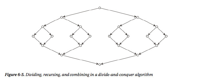
用图形来表示如下，上面部分是分(division)，下面部分是合(combination)

二分查找是最常用的采用分治策略的算法，我们经常使用的版本控制系统(evision control systems=RCSs)查找代码中发生某个变化是在哪个版本时采用的正是二分查找策略。

Python中bisect模块也正是利用了二分查找策略，其中方法bisect的作用是返回要找到元素的位置，bisect_left是其左边的那个位置，而bisect_right和bisect的作用是一样的，函数insort也是这样设计的。

Python

from bisect import bisect
a = [0, 2, 3, 5, 6, 7, 8, 8, 9]
print bisect(a, 5) #4
from bisect import bisect_left, bisect_right
print bisect_left(a, 5) #3
print bisect_right(a, 5) #4

二分查找策略很好，但是它有个前提，序列必须是有序的才可以这样做，为了高效地得到中间位置的元素，于是就有了二叉搜索树，这个我们在数据结构篇中已经详细介绍过了，下面给出一份完整的二叉搜索树的实现，不过多介绍了。

Python

class Node:
    lft = None
    rgt = None
    def __init__(self, key, val):
        self.key = key
        self.val = val

def insert(node, key, val):
    if node is None: return Node(key, val)      # Empty leaf: Add node here
    if node.key == key: node.val = val          # Found key: Replace val
    elif key < node.key:                        # Less than the key?
        node.lft = insert(node.lft, key, val)   # Go left
    else:                                       # Otherwise...
        node.rgt = insert(node.rgt, key, val)   # Go right
    return node

def search(node, key):
    if node is None: raise KeyError             # Empty leaf: It's not here
    if node.key == key: return node.val         # Found key: Return val
    elif key < node.key:                        # Less than the key?
        return search(node.lft, key)            # Go left
    else:                                       # Otherwise...
        return search(node.rgt, key)            # Go right

class Tree:                                     # Simple wrapper
    root = None
    def __setitem__(self, key, val):
        self.root = insert(self.root, key, val)
    def __getitem__(self, key):
        return search(self.root, key)
    def __contains__(self, key):
        try: search(self.root, key)
        except KeyError: return False
        return True

比较：二分法，二叉搜索树，字典

三者都是用来提高搜索效率的，但是各有区别。二分法只能作用于有序数组(例如排序后的Python的list)，但是有序数组较难维护，因为插入需要线性时间；二叉搜索树有些复杂，动态变化着，但是插入和删除效率高了些；字典的效率相比而言就比较好了，插入删除操作的平均时间都是常数的，只不过它还需要计算下hash值才能确定元素的位置。

3.顺序统计量

在算法导论中一组序列中的第 k 大的元素定义为顺序统计量

如果我们想要在线性时间内找到一组序列中的前 k 大的元素怎么做呢？很显然，如果这组序列中的数字范围比较大的话，我们就不能使用线性排序算法，而其他的基于比较的排序算法的最好的平均时间复杂度(O(nlgn))都超过了线性时间，怎么办呢？

[扩展知识：在Python中如果泥需要求前 k 小或者前 k 大的元素，可以使用heapq模块中的nsmallest或者nlargest函数，如果 k 很小的话这种方式会好些，但是如果 k 很大的话，不如直接去调用sort函数]

要想解决这个问题，我们还是要用分治法，采用类似快排中的partition将序列进行划分(divide)，也就是说找一个主元(pivot)，然后用主元作为基准将序列分成两部分，一部分小于主元，另一半大于主元，比较下主元最终的位置值和 k的大小关系，然后确定后面在哪个部分继续进行划分。如果这里不理解的话请移步阅读前面数据结构篇之排序中的快速排序

基于上面的想法就有了下面的实现，需要注意的是下面的partition函数不是就地划分的哟

Python

#A Straightforward Implementation of Partition and Select
def partition(seq):
    pi, seq = seq[0], seq[1:]                   # Pick and remove the pivot
    lo = [x for x in seq if x <= pi]            # All the small elements
    hi = [x for x in seq if x > pi]             # All the large ones
    return lo, pi, hi                           # pi is "in the right place"

def select(seq, k):
    lo, pi, hi = partition(seq)                 # [<= pi], pi, [> pi]
    m = len(lo)
    if m == k: return pi                        # We found the kth smallest
    elif m < k:                                 # Too far to the left
        return select(hi, k-m-1)                # Remember to adjust k
    else:                                       # Too far to the right
        return select(lo, k)                    # Just use original k here

seq = [3, 4, 1, 6, 3, 7, 9, 13, 93, 0, 100, 1, 2, 2, 3, 3, 2]
print partition(seq) #([1, 3, 0, 1, 2, 2, 3, 3, 2], 3, [4, 6, 7, 9, 13, 93, 100])
print select([5, 3, 2, 7, 1], 3) #5
print select([5, 3, 2, 7, 1], 4) #7
ans = [select(seq, k) for k in range(len(seq))]
seq.sort()
print ans == seq #True

细读上面的代码发现主元默认就是第一个元素，你也许会想这么选科学吗？事实证明这种随机选择的期望运行时间的确是线性的，但是如果每次都选择的不好，导致划分的时候每次都特别不平衡将会导致运行时间变成平方时间，那有没有什么选主元的办法能够保证算法的运行时间是线性的？的确有！但是比较麻烦，实际使用的并不多，感兴趣可以看下面的内容

[我还未完全理解，算法导论上也有相应的介绍，感兴趣不妨去阅读下]

It turns out guaranteeing that the pivot is even a small percentage into the sequence (that is, not at either end, or a constant number of steps from it) is enough for the running time to be linear. In 1973, a group of algorists (Blum, Floyd, Pratt, Rivest, and Tarjan) came up with a version of the algorithm that gives exactly this kind of guarantee.

The algorithm is a bit involved, but the core idea is simple enough: first divide the sequence into groups of five (or some other small constant). Find the median in each, using (for example) a simple sorting algorithm. So far, we’ve used only linear time. Now, find the median among these medians, using the linear selection algorithm recursively. (This will work, because the number of medians is smaller than the size of the original sequence—still a bit mind-bending.) The resulting value is a pivot that is guaranteed to be good enough to avoid the degenerate recursion—use it as a pivot in your selection.

In other words, the algorithm is used recursively in two ways: first, on the sequence of medians, to find a good pivot, and second, on the original sequence, using this pivot.

While the algorithm is important to know about for theoretical reasons (because it means selection can be done in guaranteed linear time), you’ll probably never actually use it in practice.

3.二分排序

前面我们介绍了二分查找，下面看看如何进行二分排序，这里不再详细介绍快排和合并排序的思想了，如果不理解的话请移步阅读前面数据结构篇之排序

利用前面的partition函数快排代码呼之欲出

Python

def quicksort(seq):
    if len(seq) <= 1: return seq                # Base case
    lo, pi, hi = partition(seq)                 # pi is in its place
    return quicksort(lo) + [pi] + quicksort(hi) # Sort lo and hi separately

seq = [7, 5, 0, 6, 3, 4, 1, 9, 8, 2]
print quicksort(seq) #[0, 1, 2, 3, 4, 5, 6, 7, 8, 9]

合并排序是更加典型的采用分治法策略来进行的排序，注意后半部分是比较谁大然后调用append函数，最后reverse一下，因为如果是比较谁小的话就要调用insert函数，它的效率不如append


Python

# Mergesort, repeated from Chapter 3 (with some modifications)
def mergesort(seq):
    mid = len(seq)//2                           # Midpoint for division
    lft, rgt = seq[:mid], seq[mid:]
    if len(lft) > 1: lft = mergesort(lft)       # Sort by halves
    if len(rgt) > 1: rgt = mergesort(rgt)
    res = []
    while lft and rgt:                          # Neither half is empty
        if lft[-1] >= rgt[-1]:                  # lft has greatest last value
            res.append(lft.pop())               # Append it
        else:                                   # rgt has greatest last value
            res.append(rgt.pop())               # Append it
    res.reverse()                               # Result is backward
    return (lft or rgt) + res                   # Also add the remainder

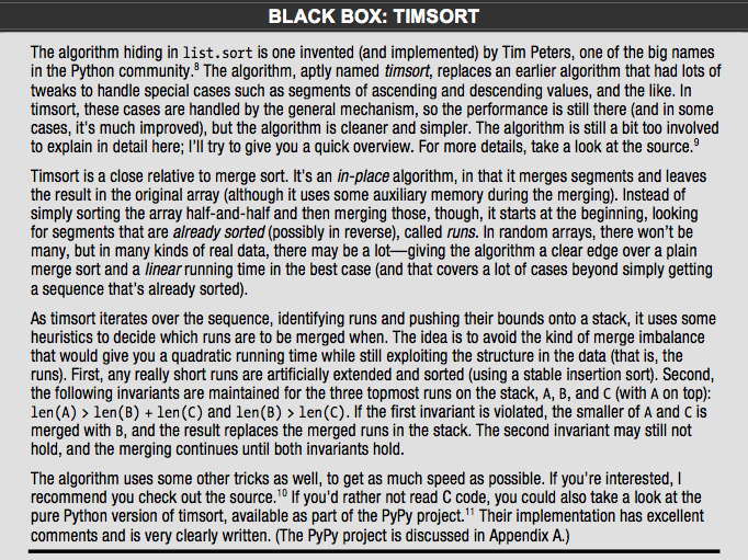
[扩展知识：Python内置的排序算法TimSort，看起来好复杂的样子啊，我果断只是略读了一下下]

[章节最后作者介绍了一些关于树平衡的内容，提到2-3树，我对树平衡不是特别感兴趣，也不是很明白，所以跳过不总结，感兴趣的不妨阅读下]

---

问题6-2. 三分查找

Binary search divides the sequence into two approximately equal parts in each recursive step. Consider ternary search, which divides the sequence into three parts. What would its asymptotic complexity be? What can you say about the number of comparisons in binary and ternary search?

题目就是说让我们分析下三分查找的时间复杂度，和二分查找进行下对比

The asymptotic running time would be the same. The number of comparison goes up, however. To see this, consider the recurrences B(n) = B(n/2) + 1 and T(n) = T(n/3) + 2 for binary and ternary search, respectively (with base cases B(1) = T(1) = 0 and B(2) = T(2) = 1). You can show (by induction) that B(n) < lg n + 1 < T(n).