Python算法:图,python算法, [The shorte
Python算法:图,python算法, [The shorte
本节主要介绍图算法中的各种最短路径算法,从不同的角度揭示它们的内核以及它们的异同
在前面的内容里我们已经介绍了图的表示方法(邻接矩阵和“各种”邻接表)、图的遍历(DFS和BFS)、图中的一些基本算法(基于DFS的拓扑排序和有向无环图的强连通分量、最小生成树的Prim和Kruskal算法等),剩下的就是图算法中的各种最短路径算法,也就是本节的主要内容。
[The shortest path problem comes in several varieties. For example, you can find shortest paths (just like any other kinds of paths) in both directed and undirected graphs. The most important distinctions, though, stem from your starting points and destinations. Do you want to find the shortest from one node to all others (single source)? From one node to another (single pair, one to one, point to point)? From all nodes to one (single destination)? From all nodes to all others (all pairs)? Two of these—single source and all pairs—are perhaps the most important. Although we have some tricks for the single pair problem (see “Meeting in the middle” and “Knowing where you’re going,” later), there are no guarantees that will let us solve that problem any faster than the general single source problem. The single destination problem is, of course, equivalent (just flip the edges for the directed case). The all pairs problem can be tackled by using each node as a single source (and we’ll look into that), but there are special-purpose algorithms for that problem as well.]
最短路径问题有很多的变种,比如我们是处理有向图还是无向图上的最短路径问题呢?此外,各个问题之间最大的区别在于起点和终点。这个问题是从一个节点到所有其他节点的最短路径吗(单源最短路径)?还是从一个节点到另一个节点的最短路径(单对节点间最短路径)?还是从所有其他节点到某一个节点(多源最短路径)?还是求任何两个节点之间的最短路径(所有节点对最短路径)?
其中单源最短路径和所有节点对最短路径是最常见的问题类型,其他问题大致可以将其转化成这两类问题。虽然单对节点间最短路径问题有一些求解的技巧(“Meeting in the middle” and “Knowing where you’re going,”),但是该问题并没有比单源最短路径问题的解法快到哪里去,所以单对节点间最短路径问题可以就用单源最短路径问题的算法去求解;而多源点单终点的最短路径问题可以将边反转过来看成是单源最短路径问题;至于所有节点对最短路径问题,可以对图中的每个节点使用单源最短路径来求解,但是对于这个问题还有一些特殊的更好的算法可以解决。
在开始介绍各种算法之前,作者给出了图中的几个重要结论或者性质,此处附上原文
assume that we start in node s and that we initialize D[s] to zero, while all other distance estimates are set to infinity. Let d(u,v) be the length of the shortest path from u to v.
• d(s,v) <= d(s,u) + W[u,v]. This is an example of the triangle inequality.
• d(s,v) <= D[v]. For v other than s, D[v] is initially infinite, and we reduce it only when we find actual shortcuts. We never “cheat,” so it remains an upper bound.
• If there is no path to node v, then relaxing will never get D[v] below infinity. That’s because we’ll never find any shortcuts to improve D[v].
• Assumeashortestpathtovisformedbyapathfromstouandanedgefromutov. Now, if D[u] is correct at any time before relaxing the edge from u to v, then D[v] is correct at all times afterward. The path defined by P[v] will also be correct.
• Let [s, a, b, … , z, v] be a shortest path from s to v. Assume all the edges (s,a), (a,b), … , (z,v) in the path have been relaxed in order. Then D[v] and P[v] will be correct. It doesn’t matter if other relax operations have been performed in between.
[最后这个是路径松弛性质,也就是后面的Bellman-Ford算法的核心]
对于单对节点间最短路径问题,如果每条边的权值都一样(或者说边一样长)的话,使用前面的BFS就可以得到结果了(第5节遍历中介绍了);如果图是有向无环图,那么我们还可以用前面动规中的DAG最短路径算法来求解(第8节动态规划中介绍了),但是,现实中的图总是有环的,边的权值也总是不同,而且可能有负权值,所以我们还需要其他的算法!
首先我们来实现下之前学过的松弛技术relaxtion,代码中D保存各个节点到源点的距离值估计(上界值),P保存节点的最短路径上的前驱节点,W保存边的权值,其中不存在的边的权值为inf。松弛就是说,假设节点 u 和节点 v 事先都有一个最短距离的估计(例如测试代码中的7和13),如果现在要松弛边(u,v),也就是对从节点 u 通过边(u,v)到达节点 v,将这条路径得到节点 v 的距离估计值(7+3=10)和原来的节点 v 的距离估计值(13)进行比较,如果前者更小的话,就表示我们可以放弃在这之前确定的从源点到节点 v 的最短路径,改成从源点到节点 u,然后节点 u 再到节点 v,这条路线距离会更短些,这也就是发生了一次松弛!(测试代码中10<13,所以要进行松弛,此时D[v]变成10,而它的前驱节点也变成了 u)
Python
#relaxtion
inf = float('inf')
def relax(W, u, v, D, P):
    d = D.get(u,inf) + W[u][v]                  # Possible shortcut estimate
    if d < D.get(v,inf):                        # Is it really a shortcut?
        D[v], P[v] = d, u                       # Update estimate and parent
        return True                             # There was a change!

#测试代码
u = 0; v = 1
D, W, P = {}, {u:{v:3}}, {}
D[u] = 7
D[v] = 13
print D[u] # 7
print D[v] # 13
print W[u][v] # 3
relax(W, u, v, D, P) # True
print D[v] # 10
D[v] = 8
relax(W, u, v, D, P)
print D[v] # 8
显然,如果你随机地对边进行松弛,那么与该边有关的节点的距离估计值就会慢慢地变得更加准确,这样的改进会在整个图中进行传播,如果一直这么松弛下去的话,最终整个图所有节点的距离值都不会发生变化的时候我们就得到了从源点到所有节点的最短路径值。
每次松弛可以看作是向最终解前进了“一步”,我们的目标自然是希望松弛的次数越少越好,关键就是要确定松弛的次数和松弛的顺序(好的松弛顺序可以让我们直接朝着最优解前进,缩短算法运行时间),后面要介绍的图中的Bellman-Ford算法、Dijkstra算法以及DAG上的最短路径问题都是如此。
现在我们考虑一个问题,如果我们对图中的所有边都松弛一遍会怎样?可能部分顶点的距离估计值有所减小对吧,那如果再对图中的所有边都松弛一遍又会怎样呢?可能又有部分顶点的距离估计值有所减小对吧,那到底什么时候才会没有改进呢?到底什么时候可以停止了呢?
这个问题可以这么想,假设从源点 s 到节点 v 的最短路径是p=<v0, v1, v2, v3 ... vk>,此时v0=s, vk=v,那除了源点 s 之外,这条路径总共经过了其他 k 个顶点对吧,k 肯定小于 (V-1) 对吧,也就是说从节点 s 到节点 v 要经过一条最多只有(V-1)条边的路径,因为每遍松弛都是松弛所有边,那么肯定会松弛路径p 中的所有边,我们可以保险地认为第 i 次循环松弛了边<vi−1,vi>,这样的话经过 k 次松弛遍历,我们肯定能够得到节点 v 的最短路径值,再根据这条路径最多只有(V-1)条边,也就说明了我们最多只要循环地对图中的所有边都松弛(V-1)遍就可以得到所有节点的最短路径值!上面的思路就是Bellman-Ford算法了,时间复杂度是O(VE)。
下面看下算法导论上的Bellman-Ford算法的示例图
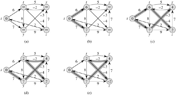
[上图的解释,需要注意的是,如果边的松弛顺序不同,可能中间得到的结果不同,但是最后的结果都是一样的:The execution of the Bellman-Ford algorithm. The source is vertex s. The d values are shown within the vertices, and shaded edges indicate predecessor values: if edge (u, v) is shaded, then π[v] = u. In this particular example, each pass relaxes the edges in the order (t, x), (t, y), (t, z), (x, t), (y, x), (y, z), (z, x), (z, s), (s, t), (s, y). (a) The situation just before the first pass over the edges. (b)-(e) The situation after each successive pass over the edges. The d and π values in part (e) are the final values. The Bellman-Ford algorithm returns TRUE in this example.]
上面的分析很好,但是我们漏考虑了一个关键问题,那就是如果图中存在负权回路的话不论我们松弛多少遍,图中有些节点的最短路径值都还是会减小,所以我们在 (V-1) 次松弛遍历之后再松弛遍历一次,如果还有节点的最短路径减小的话就说明图中存在负权回路!这就引出了Bellman-Ford算法的一个重要作用:判断图中是否存在负权回路。
Python
#Bellman-Ford算法
def bellman_ford(G, s):
    D, P = {s:0}, {}                            # Zero-dist to s; no parents
    for rnd in G:                               # n = len(G) rounds
        changed = False                         # No changes in round so far
        for u in G:                             # For every from-node...
            for v in G[u]:                      # ... and its to-nodes...
                if relax(G, u, v, D, P):        # Shortcut to v from u?
                    changed = True              # Yes! So something changed
        if not changed: break                   # No change in round: Done
    else:                                       # Not done before round n?
        raise ValueError('negative cycle')      # Negative cycle detected
    return D, P                                 # Otherwise: D and P correct

#测试代码
s, t, x, y, z = range(5)
W = {
    s: {t:6, y:7},
    t: {x:5, y:8, z:-4},
    x: {t:-2},
    y: {x:-3, z:9},
    z: {s:2, x:7}
    }
D, P = bellman_ford(W, s)
print [D[v] for v in [s, t, x, y, z]] # [0, 2, 4, 7, -2]
print s not in P # True
print [P[v] for v in [t, x, y, z]] == [x, y, s, t] # True
W[s][t] = -100
print bellman_ford(W, s)
# Traceback (most recent call last):
#         ...
# ValueError: negative cycle
前面我们在动态规划中介绍了一个DAG图中的最短路径算法,它的时间复杂度是O(V+E)的,下面我们用松弛的思路来快速回顾一下那个算法的迭代版本。因为它先对顶点进行了拓扑排序,所以它是一个典型的通过修改边松弛的顺序来提高算法运行速度的算法,也就是说,我们不是随机松弛,也不是所有边来松弛一遍,而是沿着拓扑排序得到的节点的顺序来进行松弛,怎么松弛呢?当我们到达一个节点时我们就松弛这个节点的出边,为什么这种方式能够奏效呢?
这里还是假设从源点 s 到节点 v 的最短路径是p=<v0, v1, v2, v3 ... vk>,此时v0=s, vk=v,如果我们到达了节点 v,那么说明源点 s 和节点 v 之间的那些点都已经经过了(节点是经过了拓扑排序的哟),而且它们的边也都已经松弛过了,所以根据路径松弛性质可以知道当我们到达节点 v 时我们能够直接得到源点 s 到节点 v 的最短路径值。
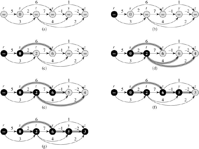
[上图的解释:The execution of the algorithm for shortest paths in a directed acyclic graph. The vertices are topologically sorted from left to right. The source vertex is s. The d values are shown within the vertices, and shaded edges indicate the π values. (a) The situation before the first iteration of the for loop of lines 3-5. (b)-(g) The situation after each iteration of the for loop of lines 3-5. The newly blackened vertex in each iteration was used as u in that iteration. The values shown in part (g) are the final values.]
接下来我们看下Dijkstra算法,它看起来非常像Prim算法,同样是基于贪心策略,每次贪心地选择松弛距离最近的“边缘节点”所在的那条边(另一个节点在已经包含的节点集合中),那为什么这种方式也能奏效呢?因为算法导论给出了完整的证明,不信你去看看!呵呵,开玩笑的啦,如果光说有证明就用不着我来写文章咯,其实是因为Dijkstra算法隐藏了一个DAG最短路径算法,而DAG的最短路径问题我们上面已经介绍过了,仔细想也不难发现,它们的区别就是松弛的顺序不同,DAG最短路径算法是先进行拓扑排序然后松弛,而Dijkstra算法是每次直接贪心地选择一条边来松弛。那为什么Dijkstra算法隐藏了一个DAG?
[这里我想了好久怎么解释,但是还是觉得原文实在太精彩,我想我这有限的水平很难讲明白,故这里附上原文,前面部分作者解释了为什么DAG最短路径算法中边松弛的顺序和拓扑排序有关,然后作者继续解释(Dijkstra算法中)下一个要加入(到已包含的节点集合)的节点必须有正确的距离估计值,最后作者解释了这个节点肯定是那个具有最小距离估计值的节点!一切顺风顺水,但是有一个重要前提条件,那就是边不能有负权值!]
作者下面的解释中提到的图9-1
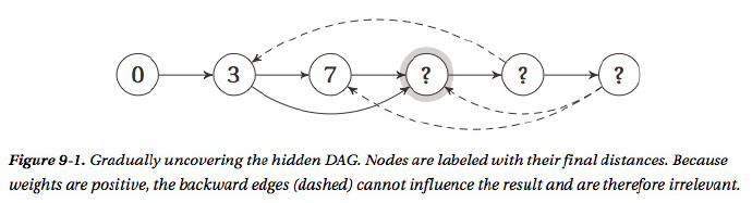
To get thing started, we can imagine that we already know the distances from the start node to each of the others. We don’t, of course, but this imaginary situation can help our reasoning. Imagine ordering the nodes, left to right, based on their distance. What happens? For the general case—not much. However, we’re assuming that we have no negative edge weights, and that makes all the difference.
Because all edges are positive, the only nodes that can contribute to a node’s solution will lie to its left in our hypothetical ordering. It will be impossible to locate a node to the right that will help us find a shortcut, because this node is further away, and could only give us a shortcut if it had a negative back edge. The positive back edges are completely useless to us, and aren’t part of the problem structure. What remains, then, is a DAG, and the topological ordering we’d like to use is exactly the hypothetical ordering we started with: nodes sorted by their actual distance. See Figure 9-1 for an illustration of this structure. (I’ll get back to the question marks in a minute.)
Predictably enough, we now hit the major gap in the solution: it’s totally circular. In uncovering the basic problem structure (decomposing into subproblems or finding the hidden DAG), we’ve assumed that we’ve already solved the problem. The reasoning has still been useful, though, because we now have something specific to look for. We want to find the ordering—and we can find it with our trusty workhorse, induction!
Consider, again, Figure 9-1. Assume that the highlighted node is the one we’re trying to identify in our inductive step (meaning that the earlier ones have been identified and already have correct distance estimates). Just like in the ordinary DAG shortest path problem, we’ll be relaxing all out-edges for each node, as soon as we’ve identified it and determined its correct distance. That means that we’ve relaxed the edges out of all earlier nodes. We haven’t relaxed the out-edges of later nodes, but as discussed, they can’t matter: the distance estimates of these later nodes are upper bounds, and the back-edges have positive weights, so there’s no way they can contribute to a shortcut.
This means (by the earlier relaxation properties or the discussion of the DAG shortest path algorithm in Chapter 8) that the next node must have a correct distance estimate. That is, the highlighted node in Figure 9-1 must by now have received its correct distance estimate, because we’ve relaxed all edges out of the first three nodes. This is very good news, and all that remains is to figure out which node it is. We still don’t really know what the ordering is, remember? We’re figuring out the topological sorting as we go along, step by step.
There is only one node that could possibly be the next one, of course:3 the one with the lowest distance estimate. We know it’s next in the sorted order, and we know it has a correct estimate; because these estimates are upper bounds, none of the later nodes could possibly have lower estimates. Cool, no? And now, by induction, we’ve solved the problem. We just relax all out-edges of the nodes of each node in distance order—which means always taking the one with the lowest estimate next.
下图是算法导论中Dijkstra算法的示例图,可以参考下
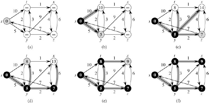
[上图的解释:The execution of Dijkstra’s algorithm. The source s is the leftmost vertex. The shortest-path estimates are shown within the vertices, and shaded edges indicate predecessor values. Black vertices are in the set S, and white vertices are in the min-priority queue Q = V – S. (a) The situation just before the first iteration of the while loop of lines 4-8. The shaded vertex has the minimum d value and is chosen as vertex u in line 5. (b)-(f) The situation after each successive iteration of the while loop. The shaded vertex in each part is chosen as vertex u in line 5 of the next iteration. The d and π values shown in part (f) are the final values.]
下面是Dijkstra算法的实现
Python
#Dijkstra算法
from heapq import heappush, heappop

def dijkstra(G, s):
    D, P, Q, S = {s:0}, {}, [(0,s)], set()      # Est., tree, queue, visited
    while Q:                                    # Still unprocessed nodes?
        _, u = heappop(Q)                       # Node with lowest estimate
        if u in S: continue                     # Already visited? Skip it
        S.add(u)                                # We've visited it now
        for v in G[u]:                          # Go through all its neighbors
            relax(G, u, v, D, P)                # Relax the out-edge
            heappush(Q, (D[v], v))              # Add to queue, w/est. as pri
    return D, P                                 # Final D and P returned

#测试代码
s, t, x, y, z = range(5)
W = {
    s: {t:10, y:5},
    t: {x:1, y:2},
    x: {z:4},
    y: {t:3, x:9, z:2},
    z: {x:6, s:7}
    }
D, P = dijkstra(W, s)
print [D[v] for v in [s, t, x, y, z]] # [0, 8, 9, 5, 7]
print s not in P # True
print [P[v] for v in [t, x, y, z]] == [y, t, s, y] # True
Dijkstra算法和Prim算法的实现很像,也和BFS算法实现很像,其实,如果我们把每条权值为 w 的边(u,v)想象成节点 u 和节点 v 中间有 (w-1) 个节点,且每条边都是权值为1的一条路径的话,BFS算法其实就和Dijkstra算法差不多了。 Dijkstra算法的时间复杂度和使用的优先队列有关,上面的实现用的是最小堆,所以时间复杂度是O(mlgn),其中 m 是边数,n 是节点数。
下面我们来看看所有点对最短路径问题
对于所有点对最短路径问题,我们第一个想法肯定是对每个节点运行一遍Dijkstra算法就可以了嘛,但是,Dijkstra算法有个前提条件,所有边的权值都是正的,那些包含了负权边的图怎么办?那就想办法对图进行些预处理,使得所有边的权值都是正的就可以了,那怎么处理能够做到呢?此时可以看下前面的三角不等性质,内容如下:
d(s,v) <= d(s,u) + W[u,v]. This is an example of the triangle inequality.
令h(u)=d(s,u), h(v)=d(s,v),假设我们给边(u,v)重新赋权w’(u, v) = w(u, v) + h(u) – h(v),根据三角不等性质可知w’(u, v)肯定非负,这样新图的边就满足Dijkstra算法的前提条件,但是,我们怎么得到每个节点的最短路径值d(s,v)?
其实这个问题很好解决对吧,前面介绍的Bellman-Ford算法就干这行的,但是源点 s 是什么?这里的解决方案有点意思,我们可以向图中添加一个顶点 s,并且让它连接图中的所有其他节点,边的权值都是0,完了之后我们就可以在新图上从源点 s 开始运行Bellman-Ford算法,这样就得到了每个节点的最短路径值d(s,v)。但是,新的问题又来了,这么改了之后真的好吗?得到的最短路径对吗?
这里的解释更加有意思,想想任何一条从源点 s 到节点 v 的路径p=<s, v1, v2, v3 ... u, v>,假设我们把路径上的边权值都加起来的话,你会发现下面的有意思的现象(telescoping sums):
sum=[w(s,v1)+h(s)-h(v1)]+[w(v1,v2)+h(v1)-h(v2)]+…+[w(u,v)+h(u)-h(v)] =w(v1,v2)+w(v2,v3)+…+w(u,v)-h(v)
上面的式子说明,所有从源点 s 到节点 v 的路径都会减去h(v),也就说明对于新图上的任何一条最短路径,它都是对应着原图的那条最短路径,只是路径的权值减去了h(v),这也就说明采用上面的策略得到的最短路径没有问题。
现在我们捋一捋思路,我们首先要使用Bellman-Ford算法得到每个节点的最短路径值,然后利用这些值修改图中边的权值,最后我们对图中所有节点都运行一次Dijkstra算法就解决了所有节点对最短路径问题,但是如果原图本来边的权值就都是正的话就直接运行Dijkstra算法就行了。这就是Johnson算法,一个巧妙地利用Bellman-Ford和Dijkstra算法结合来解决所有节点对最短路径问题的算法。它特别适合用于稀疏图,算法的时间复杂度是O(mnlgn),比后面要介绍的Floyd-Warshall算法要好些。
还有一点需要补充的是,在运行完了Dijkstra算法之后,如果我们要得到准确的最短路径的权值的话,我们还需要做一定的修改,从前面的式子可以看出,新图上节点 u 和节点 v 之间的最短路径 D’(u,v) 与原图上两个节点的最短路径 D(u,v) 有如下左式的关系,那么经过右式的简单计算就能得到原图的最短路径值
D’(u,v)=D(u,v)+h(u)-h(v) ==> D(u,v)=D’(u,v)-h(u)+h(v)
基于上面的思路,我们可以得到下面的Johnson算法实现
Python
#Johnson’s Algorithm
def johnson(G):                                 # All pairs shortest paths
    G = deepcopy(G)                             # Don't want to break original
    s = object()                                # Guaranteed unique node
    G[s] = {v:0 for v in G}                     # Edges from s have zero wgt
    h, _ = bellman_ford(G, s)                   # h[v]: Shortest dist from s
    del G[s]                                    # No more need for s
    for u in G:                                 # The weight from u...
        for v in G[u]:                          # ... to v...
            G[u][v] += h[u] - h[v]              # ... is adjusted (nonneg.)
    D, P = {}, {}                               # D[u][v] and P[u][v]
    for u in G:                                 # From every u...
        D[u], P[u] = dijkstra(G, u)             # ... find the shortest paths
        for v in G:                             # For each destination...
            D[u][v] += h[v] - h[u]              # ... readjust the distance
    return D, P                                 # These are two-dimensional

a, b, c, d, e = range(5)
W = {
    a: {c:1, d:7},
    b: {a:4},
    c: {b:-5, e:2},
    d: {c:6},
    e: {a:3, b:8, d:-4}
    }
D, P = johnson(W)
print [D[a][v] for v in [a, b, c, d, e]] # [0, -4, 1, -1, 3]
print [D[b][v] for v in [a, b, c, d, e]] # [4, 0, 5, 3, 7]
print [D[c][v] for v in [a, b, c, d, e]] # [-1, -5, 0, -2, 2]
print [D[d][v] for v in [a, b, c, d, e]] # [5, 1, 6, 0, 8]
print [D[e][v] for v in [a, b, c, d, e]] # [1, -3, 2, -4, 0]
下面我们看下Floyd-Warshall算法,这是一个基于动态规划的算法,时间复杂度是O(n3),n是图中节点数
假设所有节点都有一个数字编号(从1开始),我们要把原来的问题reduce成一个个子问题,子问题有三个参数:起点 u、终点 v、能经过的节点的最大编号k,也就是求从起点 u 到终点 v 只能够经过编号为(1,2,3,…,k)的节点的最短路径问题 (原文表述如下)
Let d(u, v, k) be the length of the shortest path that exists from node u to node v if you’re only allowed to use the k first nodes as intermediate nodes.
这个子问题怎么考虑呢?当然还是采用之前动态规划中常用的选择还是不选择这种策略,如果我们选择不经过节点 k 的话,那么问题变成了求从起点 u 到终点 v 只能够经过编号为(1,2,3,…,k-1)的节点的最短路径问题;如果我们选择经过节点 k 的话,那么问题变成求从起点 u 到终点 k 只能够经过编号为(1,2,3,…,k-1)的节点的最短路径问题与求从起点 k 到终点 v 只能够经过编号为(1,2,3,…,k-1)的节点的最短路径问题之和,如下图所示
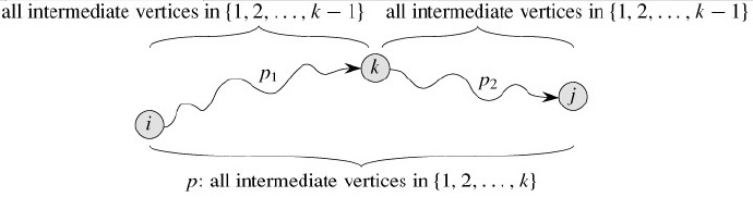
经过上面的分析,我们可以得到下面的结论
d(u,v,k) = min(d(u,v,k-1), d(u,k,k-1) + d(k,v,k-1))
根据这个式子我们很快可以得到下面的递归实现
Python
#递归版本的Floyd-Warshall算法
from functools import wraps

def memo(func):
    cache = {}                                  # Stored subproblem solutions
    @wraps(func)                                # Make wrap look like func
    def wrap(*args):                            # The memoized wrapper
        if args not in cache:                   # Not already computed?
            cache[args] = func(*args)           # Compute & cache the solution
        return cache[args]                      # Return the cached solution
    return wrap                                 # Return the wrapper

def rec_floyd_warshall(G):                                # All shortest paths
    @memo                                                 # Store subsolutions
    def d(u,v,k):                                         # u to v via 1..k
        if k==0: return G[u][v]                           # Assumes v in G[u]
        return min(d(u,v,k-1), d(u,k,k-1) + d(k,v,k-1))   # Use k or not?
    return {(u,v): d(u,v,len(G)) for u in G for v in G}   # D[u,v] = d(u,v,n)

#测试代码
a, b, c, d, e = range(1,6) # One-based
W = {
    a: {c:1, d:7},
    b: {a:4},
    c: {b:-5, e:2},
    d: {c:6},
    e: {a:3, b:8, d:-4}
    }
for u in W:
    for v in W:
        if u == v: W[u][v] = 0
        if v not in W[u]: W[u][v] = inf
D = rec_floyd_warshall(W)
print [D[a,v] for v in [a, b, c, d, e]] # [0, -4, 1, -1, 3]
print [D[b,v] for v in [a, b, c, d, e]] # [4, 0, 5, 3, 7]
print [D[c,v] for v in [a, b, c, d, e]] # [-1, -5, 0, -2, 2]
print [D[d,v] for v in [a, b, c, d, e]] # [5, 1, 6, 0, 8]
print [D[e,v] for v in [a, b, c, d, e]] # [1, -3, 2, -4, 0]
仔细看的话,不难发现这个解法和我们介绍动态规划时介绍的最长公共子序列的问题非常类似,如果还没有阅读的话不妨看下最长公共子序列问题的5种实现这篇文章,有了对最长公共子序列问题的理解,我们就很容易发现对于Floyd-Warshall算法我们也可以采用类似的方式来减小算法所需占用的空间,当然首先要将递归版本改成性能更好些的迭代版本。
Floyd-Warshall算法的递推公式
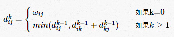
从递推公式中可以看出,计算当前回合(k)只需要上一回合(k-1)得到的结果,所以,如果应用对于中间结果不需要的话,那么可以只使用2个nxn的矩阵,一个保存当前回合(k)的结果D(k),另一个保存上一回合(k-1)的结果D(k-1),待当前回合计算完了之后将其全部复制到D(k-1)中,这样就仅需要O(n2)的空间。
Python
#空间优化后的Floyd-Warshall算法
def floyd_warshall1(G):
    D = deepcopy(G)                             # No intermediates yet
    for k in G:                                 # Look for shortcuts with k
        for u in G:
            for v in G:
                D[u][v] = min(D[u][v], D[u][k] + D[k][v])
    return D

#测试代码
a, b, c, d, e = range(1,6) # One-based
W = {
    a: {c:1, d:7},
    b: {a:4},
    c: {b:-5, e:2},
    d: {c:6},
    e: {a:3, b:8, d:-4}
    }
for u in W:
    for v in W:
        if u == v: W[u][v] = 0
        if v not in W[u]: W[u][v] = inf
D = floyd_warshall1(W)
print [D[a][v] for v in [a, b, c, d, e]] # [0, -4, 1, -1, 3]
print [D[b][v] for v in [a, b, c, d, e]] # [4, 0, 5, 3, 7]
print [D[c][v] for v in [a, b, c, d, e]] # [-1, -5, 0, -2, 2]
print [D[d][v] for v in [a, b, c, d, e]] # [5, 1, 6, 0, 8]
print [D[e][v] for v in [a, b, c, d, e]] # [1, -3, 2, -4, 0]
当然啦,一般情况下求最短路径问题我们还需要知道最短路径是什么,这个时候我们只需要在进行选择的时候设置一个前驱节点就行了
Python
#最终版本的Floyd-Warshall算法
def floyd_warshall(G):
    D, P = deepcopy(G), {}
    for u in G:
        for v in G:
            if u == v or G[u][v] == inf:
                P[u,v] = None
            else:
                P[u,v] = u
    for k in G:
        for u in G:
            for v in G:
                shortcut = D[u][k] + D[k][v]
                if shortcut < D[u][v]:
                    D[u][v] = shortcut
                    P[u,v] = P[k,v]
    return D, P

#测试代码
a, b, c, d, e = range(5)
W = {
    a: {c:1, d:7},
    b: {a:4},
    c: {b:-5, e:2},
    d: {c:6},
    e: {a:3, b:8, d:-4}
    }
for u in W:
    for v in W:
        if u == v: W[u][v] = 0
        if v not in W[u]: W[u][v] = inf
D, P = floyd_warshall(W)
print [D[a][v] for v in [a, b, c, d, e]]#[0, -4, 1, -1, 3]
print [D[b][v] for v in [a, b, c, d, e]]#[4, 0, 5, 3, 7]
print [D[c][v] for v in [a, b, c, d, e]]#[-1, -5, 0, -2, 2]
print [D[d][v] for v in [a, b, c, d, e]]#[5, 1, 6, 0, 8]
print [D[e][v] for v in [a, b, c, d, e]]#[1, -3, 2, -4, 0]
print [P[a,v] for v in [a, b, c, d, e]]#[None, 2, 0, 4, 2]
print [P[b,v] for v in [a, b, c, d, e]]#[1, None, 0, 4, 2]
print [P[c,v] for v in [a, b, c, d, e]]#[1, 2, None, 4, 2]
print [P[d,v] for v in [a, b, c, d, e]]#[1, 2, 3, None, 2]
print [P[e,v] for v in [a, b, c, d, e]]#[1, 2, 3, 4, None]
[算法导论在介绍所有节点对最短路径问题时先介绍了另一个基于动态规划的解法,但是那个算法时间复杂度较高,即使是使用了重复平方技术还是比较差,所以这里不介绍了,但是有意思的是书中将这个算法和矩阵乘法运算进行了对比,发现两者之间惊人的相似,其实同理,我们开始介绍的Bellman-Ford算法和矩阵与向量的乘法运算也有很多类似的地方,感兴趣可以自己探索下,也可以阅读算法导论了解下]
本章节最后作者还提出了两个用来解最短路径问题的技巧:“Meeting in the middle” 和 “Knowing where you’re going,”,这部分的内容又都比较难翻译和理解,感兴趣还是阅读原文较好
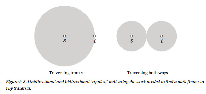
(1)Meeting in the middle
简单来说就是双向进行,Dijkstra算法是从节点 u 出发去找到达节点 v 的最短路径,但是,如果两个节点同时进行呢,当它们找到相同的节点时就得到一条路径了,这种方式比一个方向查找的效率要高些,下图是一个图示
(2)Knowing where you’re going
这里作者介绍了大名鼎鼎的A*算法,实际上也就非常类似采用了分支限界策略的BFS算法(the best-first search used in the branch and bound strategy )。
By now you’ve seen that the basic idea of traversal is pretty versatile, and by simply using different queues, you get several useful algorithms. For example, for FIFO and LIFO queues, you get BFS and DFS, and with the appropriate priorities, you get the core of Prim’s and Dijkstra’s algorithms. The algorithm described in this section, called A*, extends Dijkstra’s, by tweaking the priority once again.
As mentioned earlier, the A* algorithm uses an idea similar to Johnson’s algorithm, although for a different purpose. Johnson’s algorithm transforms all edge weights to ensure they’re positive, while ensuring that the shortest paths are still shortest. In A*, we want to modify the edges in a similar fashion, but this time the goal isn’t to make the edges positive—we’re assuming they already are (as we’re building on Dijkstra’s algorithm). No, what we want is to guide the traversal in the right direction, by using information of where we’re going: we want to make edges moving away from our target node more expensive than those that take us closer to it.
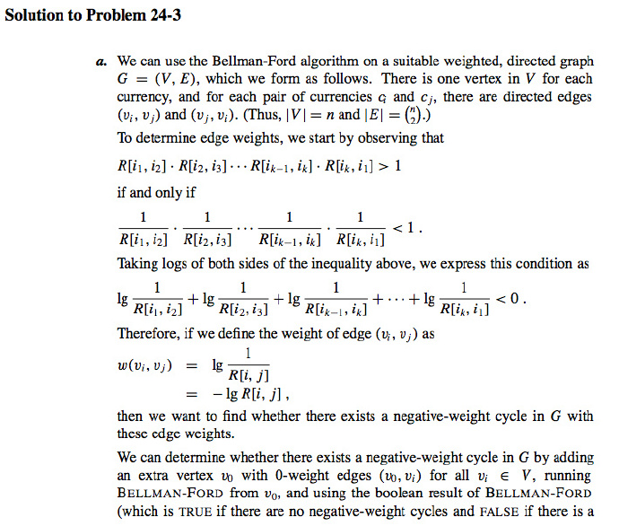
练习题:来自算法导论24-3 货币兑换问题
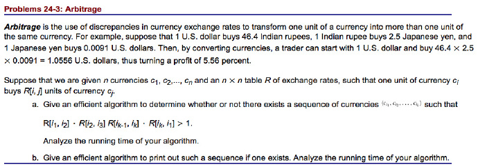
简单来说就是在给定的不同货币的兑换率下是否存在一个货币兑换循环使得最终我们能够从中获利?[提示:Bellman-Ford算法]

评论关闭