python基础2 -画图，,?#!/usr/bi

python基础2 -画图，,?#!/usr/bi

?

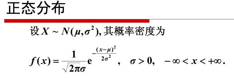
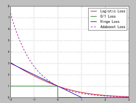
#!/usr/bin/env python# -*- coding: utf-8 -*-# Created by xuehz on 2017/4/9import numpy as npimport matplotlib as mplimport matplotlib.pyplot as pltfrom scipy.stats import norm, poissonimport timefrom scipy.optimize import leastsqfrom scipy import statsimport scipy.optimize as optimport matplotlib.pyplot as pltfrom scipy.stats import norm, poissonfrom scipy.interpolate import BarycentricInterpolatorfrom scipy.interpolate import CubicSplinefrom scipy import statsimport mathmpl.rcParams['font.sans-serif'] = [u'SimHei']  #FangSong/黑体 FangSong/KaiTimpl.rcParams['axes.unicode_minus'] = Falsedef f(x):    y = np.ones_like(x)    i = x > 0    y[i] = np.power(x[i], x[i])    i = x < 0    y[i] = np.power(-x[i], -x[i])    return ydef residual(t, x, y):    return y - (t[0] * x ** 2 + t[1] * x + t[2])def residual2(t, x, y):    print t[0], t[1]    return y - (t[0]*np.sin(t[1]*x) + t[2])if __name__ == '__main__':    #绘制正态分布概率密度函数    # mu = 0    # sigma = 1    # x = np.linspace(mu - 3 * sigma, mu + 3 * sigma, 51)    # y = np.exp(-(x - mu) ** 2 / (2 * sigma ** 2)) / (math.sqrt(2 * math.pi) * sigma)    # print x.shape    # print 'x = \n', x    # print y.shape    # print 'y = \n', y    # #plt.plot(x, y, 'ro-', linewidth=2)    # plt.figure(facecolor='w')    # plt.plot(x, y, 'r-', x, y, 'go', linewidth=2, markersize=8)    # plt.xlabel('X', fontsize=15)    # plt.ylabel('Y', fontsize=15)    # plt.title(u'高斯分布函数', fontsize=18)    # plt.grid(True)    # plt.show()    #损失函数：Logistic损失(-1,1)/SVM Hinge损失/ 0/1损失    # x = np.array(np.linspace(start=-2, stop=3, num=1001, dtype=np.float))    # y_logit = np.log(1 + np.exp(-x)) / math.log(2)    # y_boost = np.exp(-x)    # y_01 = x < 0    # y_hinge = 1.0 - x    # y_hinge[y_hinge < 0] = 0    # plt.plot(x, y_logit, 'r-', label='Logistic Loss', linewidth=2)    # plt.plot(x, y_01, 'g-', label='0/1 Loss', linewidth=2)    # plt.plot(x, y_hinge, 'b-', label='Hinge Loss', linewidth=2)    # plt.plot(x, y_boost, 'm--', label='Adaboost Loss', linewidth=2)    # plt.grid()    # plt.legend(loc='upper right')    # # plt.savefig('1.png')    # plt.show()    #x^x    # x = np.linspace(-1.3, 1.3, 101)    # y = f(x)    # plt.plot(x, y, 'g-', label='x^x', linewidth=2)    # plt.grid()    # plt.legend(loc='upper left')    # plt.show()    # #  胸型线    # x = np.arange(1, 0, -0.001)    # y = (-3 * x * np.log(x) + np.exp(-(40 * (x - 1 / np.e)) ** 4) / 25) / 2    # plt.figure(figsize=(5,7), facecolor='w')    # plt.plot(y, x, 'r-', linewidth=2)    # plt.grid(True)    # plt.title(u'胸型线', fontsize=20)    # # plt.savefig('breast.png')    # plt.show()    #    #    # # 心形线    # t = np.linspace(0, 2*np.pi, 100)    # x = 16 * np.sin(t) ** 3    # y = 13 * np.cos(t) - 5 * np.cos(2*t) - 2 * np.cos(3*t) - np.cos(4*t)    # plt.plot(x, y, 'r-', linewidth=2)    # plt.grid(True)    # plt.show()    #    # #  渐开线    # t = np.linspace(0, 50, num=1000)    # x = t*np.sin(t) + np.cos(t)    # y = np.sin(t) - t*np.cos(t)    # plt.plot(x, y, 'r-', linewidth=2)    # plt.grid()    # plt.show()    #    # # Bar    # x = np.arange(0, 10, 0.1)    # y = np.sin(x)    # plt.bar(x, y, width=0.04, linewidth=0.2)    # plt.plot(x, y, 'r--', linewidth=2)    # plt.title(u'Sin曲线')    # plt.xticks(rotation=-60)    # plt.xlabel('X')    # plt.ylabel('Y')    # plt.grid()    # plt.show()    # # # 6. 概率分布    # # 6.1 均匀分布    # x = np.random.rand(10000)    # t = np.arange(len(x))    # #plt.hist(x, 30, color='m', alpha=0.5, label=u'均匀分布')    # plt.plot(t, x, 'r-', label=u'均匀分布')    # plt.legend(loc='upper left')    # plt.grid()    # plt.show()    # # 6.2 验证中心极限定理    # t = 1000    # a = np.zeros(10000)    # for i in range(t):    #     a += np.random.uniform(-5, 5, 10000)    # a /= t    # plt.hist(a, bins=30, color='g', alpha=0.5, normed=True, label=u'均匀分布叠加')    # plt.legend(loc='upper left')    # plt.grid()    # plt.show()    #    # #6.21 其他分布的中心极限定理    # lamda = 10    # p = stats.poisson(lamda)    # y = p.rvs(size=1000)    # mx = 30    # r = (0, mx)    # bins = r[1] - r[0]    # plt.figure(figsize=(10, 8), facecolor='w')    # plt.subplot(121)    # plt.hist(y, bins=bins, range=r, color='g', alpha=0.8, normed=True)    # t = np.arange(0, mx+1)    # plt.plot(t, p.pmf(t), 'ro-', lw=2)    # plt.grid(True)    # N = 1000    # M = 10000    # plt.subplot(122)    # a = np.zeros(M, dtype=np.float)    # p = stats.poisson(lamda)    # for i in np.arange(N):    #     y = p.rvs(size=M)    #     a += y    # a /= N    # plt.hist(a, bins=20, color='g', alpha=0.8, normed=True)    # plt.grid(b=True)    # plt.show()    # # 6.3 Poisson分布    # x = np.random.poisson(lam=5, size=10000)    # print x    # pillar = 15    # a = plt.hist(x, bins=pillar, normed=True, range=[0, pillar], color='g', alpha=0.5)    # plt.grid()    # plt.show()    # print a    # print a[0].sum()    #    # # 6.4 直方图的使用    # mu = 2    # sigma = 3    # data = mu + sigma * np.random.randn(1000)    # h = plt.hist(data, 30, normed=1, color='#a0a0ff')    # x = h[1]    # y = norm.pdf(x, loc=mu, scale=sigma)    # plt.plot(x, y, 'r--', x, y, 'ro', linewidth=2, markersize=4)    # plt.grid()    # plt.show()    # # 6.5 插值    # rv = poisson(5)    # x1 = a[1]    # y1 = rv.pmf(x1)    # itp = BarycentricInterpolator(x1, y1)  # 重心插值    # x2 = np.linspace(x.min(), x.max(), 50)    # y2 = itp(x2)    # cs = scipy.interpolate.CubicSpline(x1, y1)       # 三次样条插值    # plt.plot(x2, cs(x2), 'm--', linewidth=5, label='CubicSpine')           # 三次样条插值    # plt.plot(x2, y2, 'g-', linewidth=3, label='BarycentricInterpolator')   # 重心插值    # plt.plot(x1, y1, 'r-', linewidth=1, label='Actural Value')             # 原始值    # plt.legend(loc='upper right')    # plt.grid()    # plt.show()    # 8.1 scipy    #线性回归例1    x = np.linspace(-2, 2, 50)    A, B, C = 2, 3, -1    y = (A * x ** 2 + B * x + C) + np.random.rand(len(x))*0.75    t = leastsq(residual, [0, 0, 0], args=(x, y))    theta = t[0]    print '真实值：', A, B, C    print '预测值：', theta    y_hat = theta[0] * x ** 2 + theta[1] * x + theta[2]    plt.plot(x, y, 'r-', linewidth=2, label=u'Actual')    plt.plot(x, y_hat, 'g-', linewidth=2, label=u'Predict')    plt.legend(loc='upper left')    plt.grid()    plt.show()    # 线性回归例2    x = np.linspace(0, 5, 100)    a = 5    w = 1.5    phi = -2    y = a * np.sin(w*x) + phi + np.random.rand(len(x))*0.5    t = leastsq(residual2, [3, 5, 1], args=(x, y))    theta = t[0]    print '真实值：', a, w, phi    print '预测值：', theta    y_hat = theta[0] * np.sin(theta[1] * x) + theta[2]    plt.plot(x, y, 'r-', linewidth=2, label='Actual')    plt.plot(x, y_hat, 'g-', linewidth=2, label='Predict')    plt.legend(loc='lower left')    plt.grid()    plt.show()    # marker    description    # ”.”   point    # ”,”   pixel    # “o”   circle    # “v”   triangle_down    # “^”   triangle_up    # “<”   triangle_left    # “>”   triangle_right    # “1”   tri_down    # “2”   tri_up    # “3”   tri_left    # “4”   tri_right    # “8”   octagon    # “s”   square    # “p”   pentagon    # “*”   star    # “h”   hexagon1    # “H”   hexagon2    # “+”   plus    # “x”   x    # “D”   diamond    # “d”   thin_diamond    # “|”   vline    # “_”   hline    # TICKLEFT  tickleft    # TICKRIGHT tickright    # TICKUP    tickup    # TICKDOWN  tickdown    # CARETLEFT caretleft    # CARETRIGHT    caretright    # CARETUP   caretup    # CARETDOWN caretdown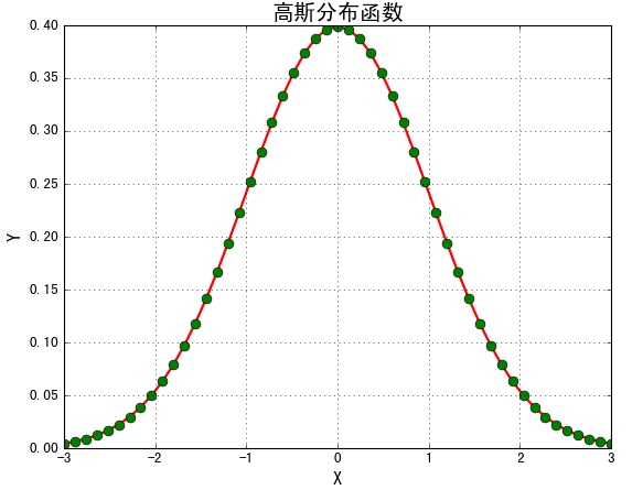

?

?

python基础2 -画图