Python时间序列分析,,Pandas生成时间
Python时间序列分析,,Pandas生成时间
Pandas生成时间序列:
import pandas as pdimport numpy as np
时间序列
时间戳(timestamp)固定周期(period)时间间隔(interval)
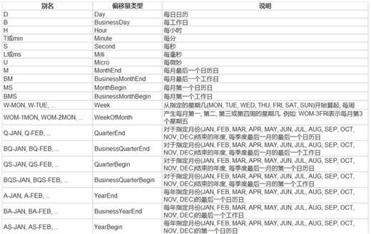
date_range
可以指定开始时间与周期H:小时D:天M:月
# TIMES的几种书写方式 #2016 Jul 1; 7/1/2016; 1/7/2016 ;2016-07-01; 2016/07/01rng = pd.date_range(‘2016-07-01‘, periods = 10, freq = ‘3D‘)#不传freq则默认是Drng
结果:


DatetimeIndex([‘2016-07-01‘, ‘2016-07-04‘, ‘2016-07-07‘, ‘2016-07-10‘, ‘2016-07-13‘, ‘2016-07-16‘, ‘2016-07-19‘, ‘2016-07-22‘, ‘2016-07-25‘, ‘2016-07-28‘], dtype=‘datetime64[ns]‘, freq=‘3D‘)View Code
time=pd.Series(np.random.randn(20), index=pd.date_range(dt.datetime(2016,1,1),periods=20))print(time)#结果:2016-01-01 -0.1293792016-01-02 0.1644802016-01-03 -0.6391172016-01-04 -0.4272242016-01-05 2.0551332016-01-06 1.1160752016-01-07 0.3574262016-01-08 0.2742492016-01-09 0.8344052016-01-10 -0.0054442016-01-11 -0.1344092016-01-12 0.2493182016-01-13 -0.2978422016-01-14 -0.1285142016-01-15 0.0636902016-01-16 -2.2460312016-01-17 0.3595522016-01-18 0.3830302016-01-19 0.4027172016-01-20 -0.694068Freq: D, dtype: float64
truncate过滤
time.truncate(before=‘2016-1-10‘)#1月10之前的都被过滤掉了
结果:
2016-01-10 -0.0054442016-01-11 -0.1344092016-01-12 0.2493182016-01-13 -0.2978422016-01-14 -0.1285142016-01-15 0.0636902016-01-16 -2.2460312016-01-17 0.3595522016-01-18 0.3830302016-01-19 0.4027172016-01-20 -0.694068Freq: D, dtype: float64View Code
time.truncate(after=‘2016-1-10‘)#1月10之后的都被过滤掉了#结果:2016-01-01 -0.1293792016-01-02 0.1644802016-01-03 -0.6391172016-01-04 -0.4272242016-01-05 2.0551332016-01-06 1.1160752016-01-07 0.3574262016-01-08 0.2742492016-01-09 0.8344052016-01-10 -0.005444Freq: D, dtype: float64
print(time[‘2016-01-15‘])#0.063690487247print(time[‘2016-01-15‘:‘2016-01-20‘])结果:2016-01-15 0.0636902016-01-16 -2.2460312016-01-17 0.3595522016-01-18 0.3830302016-01-19 0.4027172016-01-20 -0.694068Freq: D, dtype: float64data=pd.date_range(‘2010-01-01‘,‘2011-01-01‘,freq=‘M‘)print(data)#结果:DatetimeIndex([‘2010-01-31‘, ‘2010-02-28‘, ‘2010-03-31‘, ‘2010-04-30‘, ‘2010-05-31‘, ‘2010-06-30‘, ‘2010-07-31‘, ‘2010-08-31‘, ‘2010-09-30‘, ‘2010-10-31‘, ‘2010-11-30‘, ‘2010-12-31‘], dtype=‘datetime64[ns]‘, freq=‘M‘)
#时间戳pd.Timestamp(‘2016-07-10‘)#Timestamp(‘2016-07-10 00:00:00‘)# 可以指定更多细节pd.Timestamp(‘2016-07-10 10‘)#Timestamp(‘2016-07-10 10:00:00‘)pd.Timestamp(‘2016-07-10 10:15‘)#Timestamp(‘2016-07-10 10:15:00‘)# How much detail can you add?t = pd.Timestamp(‘2016-07-10 10:15‘)# 时间区间pd.Period(‘2016-01‘)#Period(‘2016-01‘, ‘M‘)pd.Period(‘2016-01-01‘)#Period(‘2016-01-01‘, ‘D‘)# TIME OFFSETSpd.Timedelta(‘1 day‘)#Timedelta(‘1 days 00:00:00‘)pd.Period(‘2016-01-01 10:10‘) + pd.Timedelta(‘1 day‘)#Period(‘2016-01-02 10:10‘, ‘T‘)pd.Timestamp(‘2016-01-01 10:10‘) + pd.Timedelta(‘1 day‘)#Timestamp(‘2016-01-02 10:10:00‘)pd.Timestamp(‘2016-01-01 10:10‘) + pd.Timedelta(‘15 ns‘)#Timestamp(‘2016-01-01 10:10:00.000000015‘)p1 = pd.period_range(‘2016-01-01 10:10‘, freq = ‘25H‘, periods = 10)p2 = pd.period_range(‘2016-01-01 10:10‘, freq = ‘1D1H‘, periods = 10)p1p2结果:PeriodIndex([‘2016-01-01 10:00‘, ‘2016-01-02 11:00‘, ‘2016-01-03 12:00‘, ‘2016-01-04 13:00‘, ‘2016-01-05 14:00‘, ‘2016-01-06 15:00‘, ‘2016-01-07 16:00‘, ‘2016-01-08 17:00‘, ‘2016-01-09 18:00‘, ‘2016-01-10 19:00‘], dtype=‘period[25H]‘, freq=‘25H‘)PeriodIndex([‘2016-01-01 10:00‘, ‘2016-01-02 11:00‘, ‘2016-01-03 12:00‘, ‘2016-01-04 13:00‘, ‘2016-01-05 14:00‘, ‘2016-01-06 15:00‘, ‘2016-01-07 16:00‘, ‘2016-01-08 17:00‘, ‘2016-01-09 18:00‘, ‘2016-01-10 19:00‘], dtype=‘period[25H]‘, freq=‘25H‘)# 指定索引rng = pd.date_range(‘2016 Jul 1‘, periods = 10, freq = ‘D‘)rngpd.Series(range(len(rng)), index = rng)结果:2016-07-01 02016-07-02 12016-07-03 22016-07-04 32016-07-05 42016-07-06 52016-07-07 62016-07-08 72016-07-09 82016-07-10 9Freq: D, dtype: int32periods = [pd.Period(‘2016-01‘), pd.Period(‘2016-02‘), pd.Period(‘2016-03‘)]ts = pd.Series(np.random.randn(len(periods)), index = periods)ts结果:2016-01 -0.0158372016-02 -0.9234632016-03 -0.485212Freq: M, dtype: float64type(ts.index)#pandas.core.indexes.period.PeriodIndex# 时间戳和时间周期可以转换ts = pd.Series(range(10), pd.date_range(‘07-10-16 8:00‘, periods = 10, freq = ‘H‘))ts结果:2016-07-10 08:00:00 02016-07-10 09:00:00 12016-07-10 10:00:00 22016-07-10 11:00:00 32016-07-10 12:00:00 42016-07-10 13:00:00 52016-07-10 14:00:00 62016-07-10 15:00:00 72016-07-10 16:00:00 82016-07-10 17:00:00 9Freq: H, dtype: int32ts_period = ts.to_period()ts_period结果:2016-07-10 08:00 02016-07-10 09:00 12016-07-10 10:00 22016-07-10 11:00 32016-07-10 12:00 42016-07-10 13:00 52016-07-10 14:00 62016-07-10 15:00 72016-07-10 16:00 82016-07-10 17:00 9Freq: H, dtype: int32时间周期与时间戳的区别ts_period[‘2016-07-10 08:30‘:‘2016-07-10 11:45‘] #时间周期包含08:00结果:2016-07-10 08:00 02016-07-10 09:00 12016-07-10 10:00 22016-07-10 11:00 3Freq: H, dtype: int32ts[‘2016-07-10 08:30‘:‘2016-07-10 11:45‘] #时间戳不包含08:30#结果:2016-07-10 09:00:00 12016-07-10 10:00:00 22016-07-10 11:00:00 3Freq: H, dtype: int32
数据重采样:
时间数据由一个频率转换到另一个频率降采样升采样import pandas as pdimport numpy as nprng = pd.date_range(‘1/1/2011‘, periods=90, freq=‘D‘)#数据按天ts = pd.Series(np.random.randn(len(rng)), index=rng)ts.head()结果:2011-01-01 -1.0255622011-01-02 0.4108952011-01-03 0.6603112011-01-04 0.7102932011-01-05 0.444985Freq: D, dtype: float64ts.resample(‘M‘).sum()#数据降采样,降为月,指标是求和,也可以平均,自己指定结果:2011-01-31 2.5101022011-02-28 0.5832092011-03-31 2.749411Freq: M, dtype: float64ts.resample(‘3D‘).sum()#数据降采样,降为3天结果:2011-01-01 0.0456432011-01-04 -2.2552062011-01-07 0.5711422011-01-10 0.8350322011-01-13 -0.3967662011-01-16 -1.1562532011-01-19 -1.2868842011-01-22 2.8839522011-01-25 1.5669082011-01-28 1.4355632011-01-31 0.3115652011-02-03 -2.5412352011-02-06 0.3170752011-02-09 1.5988772011-02-12 -1.9505092011-02-15 2.9283122011-02-18 -0.7337152011-02-21 1.6748172011-02-24 -2.0788722011-02-27 2.1723202011-03-02 -2.0221042011-03-05 -0.0703562011-03-08 1.2766712011-03-11 -2.8351322011-03-14 -1.3841132011-03-17 1.5175652011-03-20 -0.5504062011-03-23 0.7734302011-03-26 2.2443192011-03-29 2.951082Freq: 3D, dtype: float64day3Ts = ts.resample(‘3D‘).mean()day3Ts结果:2011-01-01 0.0152142011-01-04 -0.7517352011-01-07 0.1903812011-01-10 0.2783442011-01-13 -0.1322552011-01-16 -0.3854182011-01-19 -0.4289612011-01-22 0.9613172011-01-25 0.5223032011-01-28 0.4785212011-01-31 0.1038552011-02-03 -0.8470782011-02-06 0.1056922011-02-09 0.5329592011-02-12 -0.6501702011-02-15 0.9761042011-02-18 -0.2445722011-02-21 0.5582722011-02-24 -0.6929572011-02-27 0.7241072011-03-02 -0.6740352011-03-05 -0.0234522011-03-08 0.4255572011-03-11 -0.9450442011-03-14 -0.4613712011-03-17 0.5058552011-03-20 -0.1834692011-03-23 0.2578102011-03-26 0.7481062011-03-29 0.983694Freq: 3D, dtype: float64print(day3Ts.resample(‘D‘).asfreq())#升采样,要进行插值结果:2011-01-01 0.0152142011-01-02 NaN2011-01-03 NaN2011-01-04 -0.7517352011-01-05 NaN2011-01-06 NaN2011-01-07 0.1903812011-01-08 NaN2011-01-09 NaN2011-01-10 0.2783442011-01-11 NaN2011-01-12 NaN2011-01-13 -0.1322552011-01-14 NaN2011-01-15 NaN2011-01-16 -0.3854182011-01-17 NaN2011-01-18 NaN2011-01-19 -0.4289612011-01-20 NaN2011-01-21 NaN2011-01-22 0.9613172011-01-23 NaN2011-01-24 NaN2011-01-25 0.5223032011-01-26 NaN2011-01-27 NaN2011-01-28 0.4785212011-01-29 NaN2011-01-30 NaN ... 2011-02-28 NaN2011-03-01 NaN2011-03-02 -0.6740352011-03-03 NaN2011-03-04 NaN2011-03-05 -0.0234522011-03-06 NaN2011-03-07 NaN2011-03-08 0.4255572011-03-09 NaN2011-03-10 NaN2011-03-11 -0.9450442011-03-12 NaN2011-03-13 NaN2011-03-14 -0.4613712011-03-15 NaN2011-03-16 NaN2011-03-17 0.5058552011-03-18 NaN2011-03-19 NaN2011-03-20 -0.1834692011-03-21 NaN2011-03-22 NaN2011-03-23 0.2578102011-03-24 NaN2011-03-25 NaN2011-03-26 0.7481062011-03-27 NaN2011-03-28 NaN2011-03-29 0.983694Freq: D, Length: 88, dtype: float64
插值方法:
ffill 空值取前面的值bfill 空值取后面的值interpolate 线性取值day3Ts.resample(‘D‘).ffill(1)结果:2011-01-01 0.0152142011-01-02 0.0152142011-01-03 NaN2011-01-04 -0.7517352011-01-05 -0.7517352011-01-06 NaN2011-01-07 0.1903812011-01-08 0.1903812011-01-09 NaN2011-01-10 0.2783442011-01-11 0.2783442011-01-12 NaN2011-01-13 -0.1322552011-01-14 -0.1322552011-01-15 NaN2011-01-16 -0.3854182011-01-17 -0.3854182011-01-18 NaN2011-01-19 -0.4289612011-01-20 -0.4289612011-01-21 NaN2011-01-22 0.9613172011-01-23 0.9613172011-01-24 NaN2011-01-25 0.5223032011-01-26 0.5223032011-01-27 NaN2011-01-28 0.4785212011-01-29 0.4785212011-01-30 NaN ... 2011-02-28 0.7241072011-03-01 NaN2011-03-02 -0.6740352011-03-03 -0.6740352011-03-04 NaN2011-03-05 -0.0234522011-03-06 -0.0234522011-03-07 NaN2011-03-08 0.4255572011-03-09 0.4255572011-03-10 NaN2011-03-11 -0.9450442011-03-12 -0.9450442011-03-13 NaN2011-03-14 -0.4613712011-03-15 -0.4613712011-03-16 NaN2011-03-17 0.5058552011-03-18 0.5058552011-03-19 NaN2011-03-20 -0.1834692011-03-21 -0.1834692011-03-22 NaN2011-03-23 0.2578102011-03-24 0.2578102011-03-25 NaN2011-03-26 0.7481062011-03-27 0.7481062011-03-28 NaN2011-03-29 0.983694Freq: D, Length: 88, dtype: float64day3Ts.resample(‘D‘).bfill(1)结果:2011-01-01 0.0152142011-01-02 NaN2011-01-03 -0.7517352011-01-04 -0.7517352011-01-05 NaN2011-01-06 0.1903812011-01-07 0.1903812011-01-08 NaN2011-01-09 0.2783442011-01-10 0.2783442011-01-11 NaN2011-01-12 -0.1322552011-01-13 -0.1322552011-01-14 NaN2011-01-15 -0.3854182011-01-16 -0.3854182011-01-17 NaN2011-01-18 -0.4289612011-01-19 -0.4289612011-01-20 NaN2011-01-21 0.9613172011-01-22 0.9613172011-01-23 NaN2011-01-24 0.5223032011-01-25 0.5223032011-01-26 NaN2011-01-27 0.4785212011-01-28 0.4785212011-01-29 NaN2011-01-30 0.103855 ... 2011-02-28 NaN2011-03-01 -0.6740352011-03-02 -0.6740352011-03-03 NaN2011-03-04 -0.0234522011-03-05 -0.0234522011-03-06 NaN2011-03-07 0.4255572011-03-08 0.4255572011-03-09 NaN2011-03-10 -0.9450442011-03-11 -0.9450442011-03-12 NaN2011-03-13 -0.4613712011-03-14 -0.4613712011-03-15 NaN2011-03-16 0.5058552011-03-17 0.5058552011-03-18 NaN2011-03-19 -0.1834692011-03-20 -0.1834692011-03-21 NaN2011-03-22 0.2578102011-03-23 0.2578102011-03-24 NaN2011-03-25 0.7481062011-03-26 0.7481062011-03-27 NaN2011-03-28 0.9836942011-03-29 0.983694Freq: D, Length: 88, dtype: float64day3Ts.resample(‘D‘).interpolate(‘linear‘)#线性拟合填充结果:2011-01-01 0.0152142011-01-02 -0.2404352011-01-03 -0.4960852011-01-04 -0.7517352011-01-05 -0.4376972011-01-06 -0.1236582011-01-07 0.1903812011-01-08 0.2197022011-01-09 0.2490232011-01-10 0.2783442011-01-11 0.1414782011-01-12 0.0046112011-01-13 -0.1322552011-01-14 -0.2166432011-01-15 -0.3010302011-01-16 -0.3854182011-01-17 -0.3999322011-01-18 -0.4144472011-01-19 -0.4289612011-01-20 0.0344652011-01-21 0.4978912011-01-22 0.9613172011-01-23 0.8149792011-01-24 0.6686412011-01-25 0.5223032011-01-26 0.5077092011-01-27 0.4931152011-01-28 0.4785212011-01-29 0.3536322011-01-30 0.228744 ... 2011-02-28 0.2580602011-03-01 -0.2079882011-03-02 -0.6740352011-03-03 -0.4571742011-03-04 -0.2403132011-03-05 -0.0234522011-03-06 0.1262182011-03-07 0.2758872011-03-08 0.4255572011-03-09 -0.0313102011-03-10 -0.4881772011-03-11 -0.9450442011-03-12 -0.7838202011-03-13 -0.6225952011-03-14 -0.4613712011-03-15 -0.1389622011-03-16 0.1834462011-03-17 0.5058552011-03-18 0.2760802011-03-19 0.0463062011-03-20 -0.1834692011-03-21 -0.0363762011-03-22 0.1107172011-03-23 0.2578102011-03-24 0.4212422011-03-25 0.5846742011-03-26 0.7481062011-03-27 0.8266362011-03-28 0.9051652011-03-29 0.983694Freq: D, Length: 88, dtype: float64
Pandas滑动窗口:
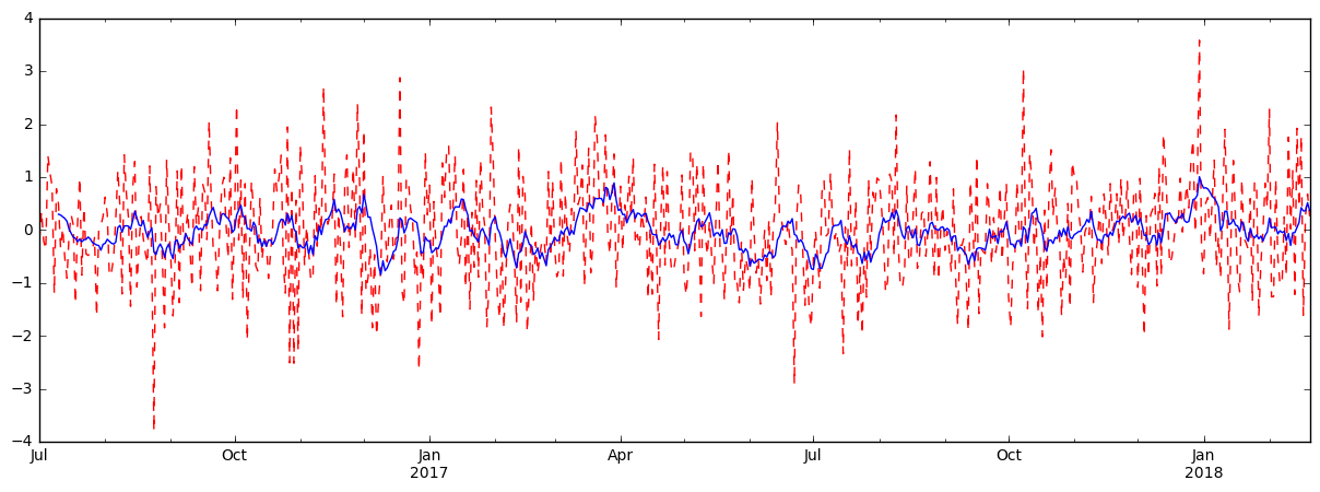
滑动窗口就是能够根据指定的单位长度来框住时间序列,从而计算框内的统计指标。相当于一个长度指定的滑块在刻度尺上面滑动,每滑动一个单位即可反馈滑块内的数据。
滑动窗口可以使数据更加平稳,浮动范围会比较小,具有代表性,单独拿出一个数据可能或多或少会离群,有差异或者错误,使用滑动窗口会更规范一些。
%matplotlib inline import matplotlib.pylabimport numpy as npimport pandas as pddf = pd.Series(np.random.randn(600), index = pd.date_range(‘7/1/2016‘, freq = ‘D‘, periods = 600))df.head()结果:2016-07-01 -0.1921402016-07-02 0.3579532016-07-03 -0.2018472016-07-04 -0.3722302016-07-05 1.414753Freq: D, dtype: float64r = df.rolling(window = 10)r#Rolling [window=10,center=False,axis=0]#r.max, r.median, r.std, r.skew倾斜度, r.sum, r.varprint(r.mean())结果:2016-07-01 NaN2016-07-02 NaN2016-07-03 NaN2016-07-04 NaN2016-07-05 NaN2016-07-06 NaN2016-07-07 NaN2016-07-08 NaN2016-07-09 NaN2016-07-10 0.3001332016-07-11 0.2847802016-07-12 0.2528312016-07-13 0.2206992016-07-14 0.1671372016-07-15 0.0185932016-07-16 -0.0614142016-07-17 -0.1345932016-07-18 -0.1533332016-07-19 -0.2189282016-07-20 -0.1694262016-07-21 -0.2197472016-07-22 -0.1812662016-07-23 -0.1736742016-07-24 -0.1306292016-07-25 -0.1667302016-07-26 -0.2330442016-07-27 -0.2566422016-07-28 -0.2807382016-07-29 -0.2898932016-07-30 -0.379625 ... 2018-01-22 -0.2114672018-01-23 0.0349962018-01-24 -0.1059102018-01-25 -0.1457742018-01-26 -0.0893202018-01-27 -0.1643702018-01-28 -0.1108922018-01-29 -0.2057862018-01-30 -0.1011622018-01-31 -0.0347602018-02-01 0.2293332018-02-02 0.0437412018-02-03 0.0528372018-02-04 0.0577462018-02-05 -0.0714012018-02-06 -0.0111532018-02-07 -0.0457372018-02-08 -0.0219832018-02-09 -0.1967152018-02-10 -0.0637212018-02-11 -0.2894522018-02-12 -0.0509462018-02-13 -0.0470142018-02-14 0.0487542018-02-15 0.1439492018-02-16 0.4248232018-02-17 0.3618782018-02-18 0.3632352018-02-19 0.5174362018-02-20 0.368020Freq: D, Length: 600, dtype: float64import matplotlib.pyplot as plt%matplotlib inlineplt.figure(figsize=(15, 5))df.plot(style=‘r--‘)df.rolling(window=10).mean().plot(style=‘b‘)#<matplotlib.axes._subplots.AxesSubplot at 0x249627fb6d8>
结果:
数据平稳性与差分法:
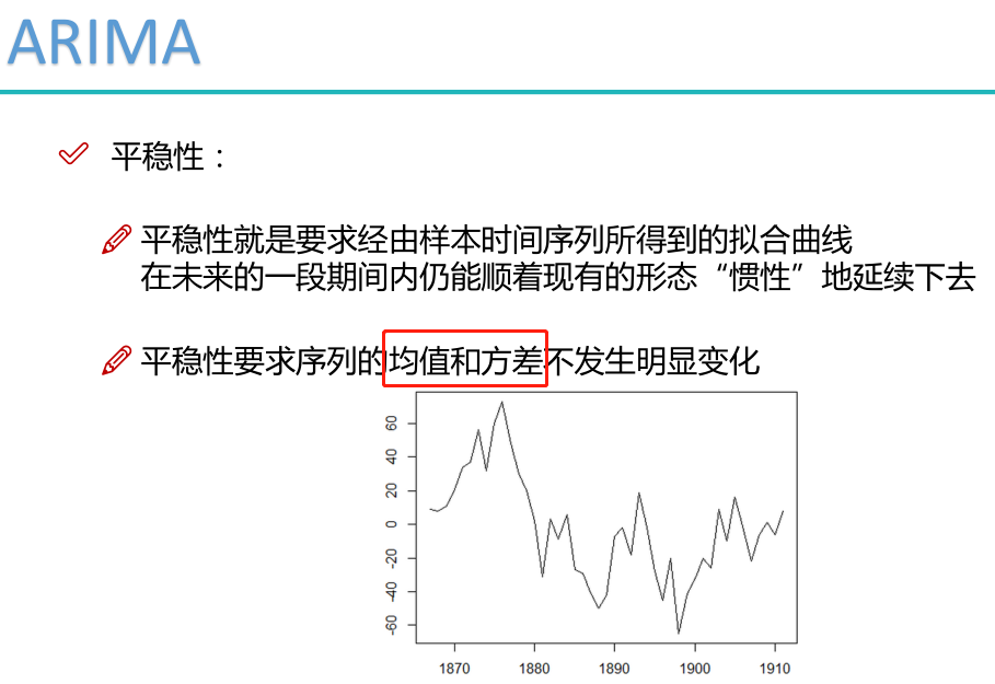

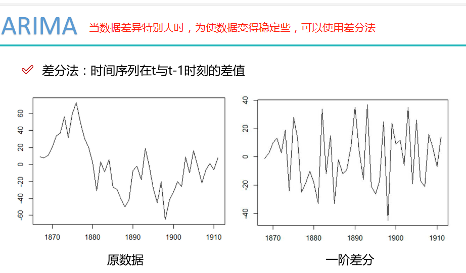
二阶差分是指在一阶差分基础上再做一阶差分。


相关函数评估方法:
Python时间序列分析
相关内容
- 分类 :kNN(k nearest neighbour)最近邻算法(Python),,
- Python知乎热门话题爬取,,本例子是参考崔老师的
- Jenkins部署python项目时,提示找不到自己定义的模块包的
- python--setUp()和tearDown()应用,,setUp:表示前置
- python中使用pip安装报错:Fatal error in launcher... 解决方法
- 使用python2连接操作db2,,在python2.6
- Python 3.6 TypeEror: iter() returned non-iterator of type,,环境:
- Mac下编译Thrift的时候Python2.7会报错 site-packages':
- Appium+Python之PO模型(Page object Model),,思考:我们进行
- python 爬虫学习--Beautiful Soup插件,,Beautiful
评论关闭