Python——sklearn提供的自带的数据集，pythonsklearn自带,sklearn提供的

Python——sklearn提供的自带的数据集，pythonsklearn自带,sklearn提供的

sklearn提供的自带的数据集

sklearn 的数据集有好多个种

自带的小数据集（packaged dataset）：sklearn.datasets.load_<name>可在线下载的数据集（Downloaded Dataset）：sklearn.datasets.fetch_<name>计算机生成的数据集（Generated Dataset）：sklearn.datasets.make_<name>svmlight/libsvm格式的数据集:sklearn.datasets.load_svmlight_file(...)从买了data.org在线下载获取的数据集:sklearn.datasets.fetch_mldata(...)

①自带的数据集

其中的自带的小的数据集为：sklearn.datasets.load_<name>

这些数据集都可以在官网上查到，以鸢尾花为例，可以在官网上找到demo，http://scikit-learn.org/stable/auto_examples/datasets/plot_iris_dataset.html

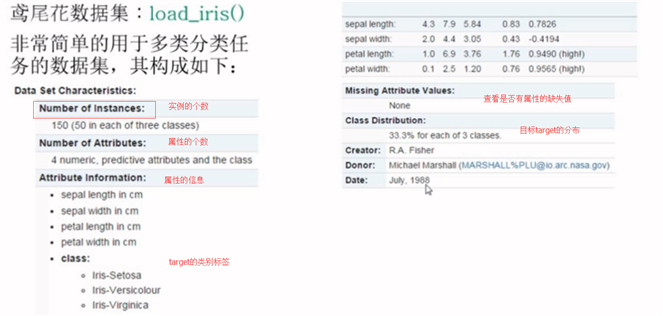
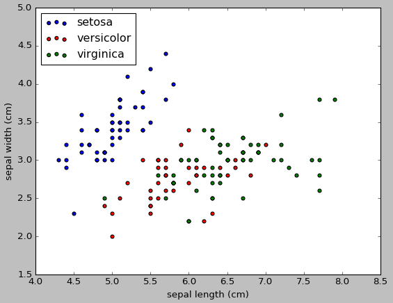
 1 from sklearn.datasets import load_iris 2 #加载数据集 3 iris=load_iris() 4 iris.keys()　　#dict_keys([‘target‘, ‘DESCR‘, ‘data‘, ‘target_names‘, ‘feature_names‘]) 5 #数据的条数和维数 6 n_samples,n_features=iris.data.shape 7 print("Number of sample:",n_samples)  #Number of sample: 150 8 print("Number of feature",n_features)　　#Number of feature 4 9 #第一个样例10 print(iris.data[0])　　　　　　#[ 5.1  3.5  1.4  0.2]11 print(iris.data.shape)　　　　#(150, 4)12 print(iris.target.shape)　　#(150,)13 print(iris.target)14 """15 16 　　[0 0 0 0 0 0 0 0 0 0 0 0 0 0 0 0 0 0 0 0 0 0 0 0 0 0 0 0 0 0 0 0 0 0 0 0 017 0 0 0 0 0 0 0 0 0 0 0 0 1 1 1 1 1 1 1 1 1 1 1 1 1 1 1 1 1 1 1 1 1 1 1 118 1 1 1 1 1 1 1 1 1 1 1 1 1 1 1 1 1 1 1 1 1 1 1 1 1 2 2 2 2 2 2 2 2 2 2 219 2 2 2 2 2 2 2 2 2 2 2 2 2 2 2 2 2 2 2 2 2 2 2 2 2 2 2 2 2 2 2 2 2 2 2 220 2]21 22 """23 import numpy as np24 print(iris.target_names)　　#[‘setosa‘ ‘versicolor‘ ‘virginica‘]25 np.bincount(iris.target)　　#[50 50 50]26 27 import matplotlib.pyplot as plt28 #以第3个索引为划分依据，x_index的值可以为0，1，2，329 x_index=330 color=[‘blue‘,‘red‘,‘green‘]31 for label,color in zip(range(len(iris.target_names)),color):32     plt.hist(iris.data[iris.target==label,x_index],label=iris.target_names[label],color=color)33 34 plt.xlabel(iris.feature_names[x_index])35 plt.legend(loc="Upper right")36 plt.show()37 38 #画散点图，第一维的数据作为x轴和第二维的数据作为y轴39 x_index=040 y_index=141 colors=[‘blue‘,‘red‘,‘green‘]42 for label,color in zip(range(len(iris.target_names)),colors):43     plt.scatter(iris.data[iris.target==label,x_index],44                 iris.data[iris.target==label,y_index],45                 label=iris.target_names[label],46                 c=color)47 plt.xlabel(iris.feature_names[x_index])48 plt.ylabel(iris.feature_names[y_index])49 plt.legend(loc=‘upper left‘)50 plt.show()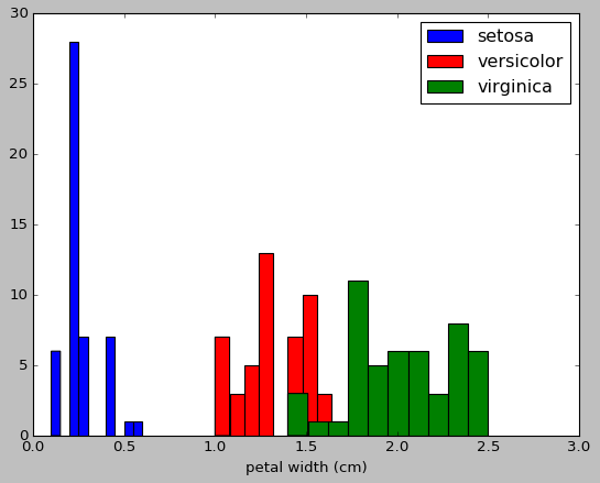

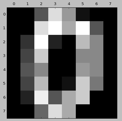
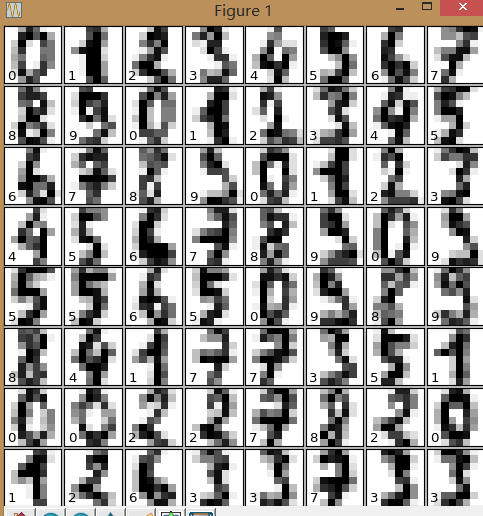
手写数字数据集load_digits()：用于多分类任务的数据集

 1 from sklearn.datasets import load_digits 2 digits=load_digits() 3 print(digits.data.shape) 4 import matplotlib.pyplot as plt 5 plt.gray() 6 plt.matshow(digits.images[0]) 7 plt.show() 8  9 from sklearn.datasets import load_digits10 digits=load_digits()11 digits.keys()12 n_samples,n_features=digits.data.shape13 print((n_samples,n_features))14 15 print(digits.data.shape)16 print(digits.images.shape)17 18 import numpy as np19 print(np.all(digits.images.reshape((1797,64))==digits.data))20 21 fig=plt.figure(figsize=(6,6))22 fig.subplots_adjust(left=0,right=1,bottom=0,top=1,hspace=0.05,wspace=0.05)23 #绘制数字：每张图像8*8像素点24 for i in range(64):25     ax=fig.add_subplot(8,8,i+1,xticks=[],yticks=[])26     ax.imshow(digits.images[i],cmap=plt.cm.binary,interpolation=‘nearest‘)27     #用目标值标记图像28     ax.text(0,7,str(digits.target[i]))29 plt.show()

乳腺癌数据集load-barest-cancer（）：简单经典的用于二分类任务的数据集

糖尿病数据集：load-diabetes（）：经典的用于回归任务的数据集，值得注意的是，这10个特征中的每个特征都已经被处理成0均值，方差归一化的特征值

波士顿房价数据集：load-boston（）：经典的用于回归任务的数据集

体能训练数据集：load-linnerud（）：经典的用于多变量回归任务的数据集，其内部包含两个小数据集：Excise是对3个训练变量的20次观测（体重，腰围，脉搏），physiological是对3个生理学变量的20次观测（引体向上，仰卧起坐，立定跳远）

svmlight/libsvm的每一行样本的存放格式：

<label><feature-id>:<feature-value><feature-id>:<feature-value> ....

这种格式比较适合用来存放稀疏数据，在sklearn中，用scipy sparse CSR矩阵来存放X，用numpy数组来存放Y

1 from sklearn.datasets import load_svmlight_file2 x_train,y_train=load_svmlight_file("/path/to/train_dataset.txt","")#如果要加在多个数据的时候，可以用逗号隔开

②生成数据集

生成数据集：可以用来分类任务，可以用来回归任务，可以用来聚类任务，用于流形学习的，用于因子分解任务的

用于分类任务和聚类任务的：这些函数产生样本特征向量矩阵以及对应的类别标签集合

make_blobs：多类单标签数据集，为每个类分配一个或多个正太分布的点集

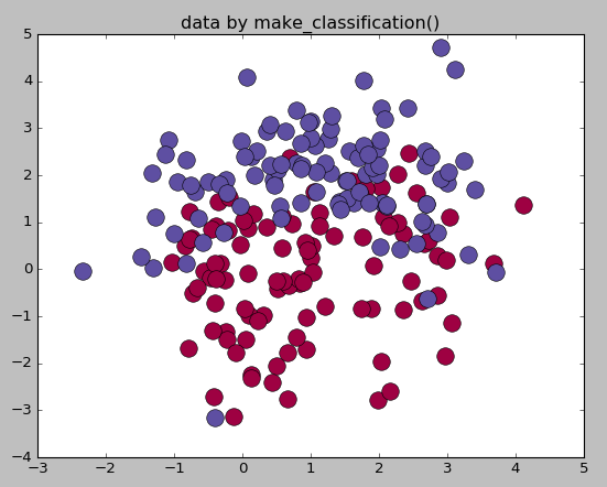
make_classification：多类单标签数据集，为每个类分配一个或多个正太分布的点集，提供了为数据添加噪声的方式，包括维度相关性，无效特征以及冗余特征等

make_gaussian-quantiles：将一个单高斯分布的点集划分为两个数量均等的点集，作为两类

make_hastie-10-2：产生一个相似的二元分类数据集，有10个维度

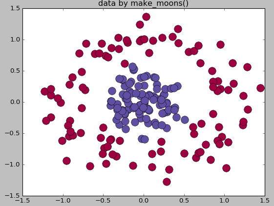
make_circle和make_moom产生二维二元分类数据集来测试某些算法的性能，可以为数据集添加噪声，可以为二元分类器产生一些球形判决界面的数据

 1 #生成多类单标签数据集 2 import numpy as np 3 import matplotlib.pyplot as plt 4 from sklearn.datasets.samples_generator import make_blobs 5 center=[[1,1],[-1,-1],[1,-1]] 6 cluster_std=0.3 7 X,labels=make_blobs(n_samples=200,centers=center,n_features=2, 8                     cluster_std=cluster_std,random_state=0) 9 print(‘X.shape‘,X.shape)10 print("labels",set(labels))11 12 unique_lables=set(labels)13 colors=plt.cm.Spectral(np.linspace(0,1,len(unique_lables)))14 for k,col in zip(unique_lables,colors):15     x_k=X[labels==k]16     plt.plot(x_k[:,0],x_k[:,1],‘o‘,markerfacecolor=col,markeredgecolor="k",17              markersize=14)18 plt.title(‘data by make_blob()‘)19 plt.show()20 21 #生成用于分类的数据集22 from sklearn.datasets.samples_generator import make_classification23 X,labels=make_classification(n_samples=200,n_features=2,n_redundant=0,n_informative=2,24                              random_state=1,n_clusters_per_class=2)25 rng=np.random.RandomState(2)26 X+=2*rng.uniform(size=X.shape)27 28 unique_lables=set(labels)29 colors=plt.cm.Spectral(np.linspace(0,1,len(unique_lables)))30 for k,col in zip(unique_lables,colors):31     x_k=X[labels==k]32     plt.plot(x_k[:,0],x_k[:,1],‘o‘,markerfacecolor=col,markeredgecolor="k",33              markersize=14)34 plt.title(‘data by make_classification()‘)35 plt.show()36 37 #生成球形判决界面的数据38 from sklearn.datasets.samples_generator import make_circles39 X,labels=make_circles(n_samples=200,noise=0.2,factor=0.2,random_state=1)40 print("X.shape:",X.shape)41 print("labels:",set(labels))42 43 unique_lables=set(labels)44 colors=plt.cm.Spectral(np.linspace(0,1,len(unique_lables)))45 for k,col in zip(unique_lables,colors):46     x_k=X[labels==k]47     plt.plot(x_k[:,0],x_k[:,1],‘o‘,markerfacecolor=col,markeredgecolor="k",48              markersize=14)49 plt.title(‘data by make_moons()‘)50 plt.show()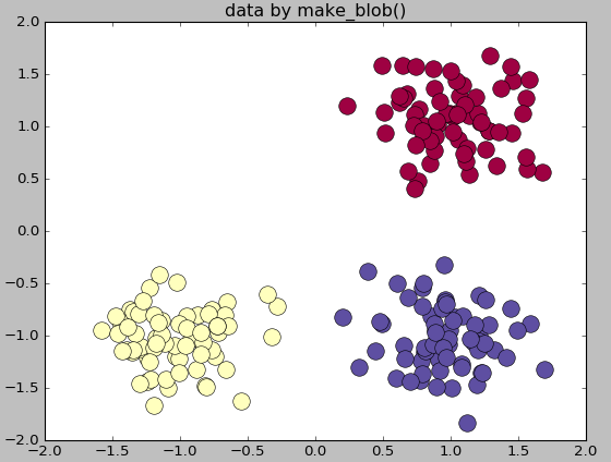

Python——sklearn提供的自带的数据集